Prerequisites: ch001–ch006
You will learn:
How to design a computational experiment: hypothesis, controls, measurement, interpretation
The difference between an experiment and a demonstration
How to measure something you cannot observe directly via proxy metrics
Common pitfalls: confirmation bias, overfitting an experiment, ignoring variance
Environment: Python 3.x, numpy, matplotlib
1. Concept
A demonstration shows that something works in one case. An experiment measures how and why it works — or doesn’t — across systematically varied conditions.
Most programmers write demonstrations. They run their algorithm on a test input, see it produce the right output, and conclude it is correct. A mathematician (and a scientist) runs experiments: vary the input systematically, measure the outcome, control for confounders, and draw quantified conclusions.
Computational experiments apply the scientific method to mathematical and algorithmic questions:
Hypothesis: a precise, falsifiable claim
Design: which variables to vary, which to hold fixed, how to measure the outcome
Execution: run the experiment, collect data
Analysis: quantify the result, estimate uncertainty
Conclusion: what the data supports — and what it does not
Common misconception: A successful run proves an algorithm correct.
One run proves nothing. It is consistent with correctness. Experiments that vary inputs, stress edge cases, and measure failure rates build genuine evidence.
2. Intuition & Mental Models
Physical analogy: Drug trials. A single patient recovering after taking a drug proves nothing — they might have recovered anyway. A randomized controlled trial with 1000 patients, a placebo group, and blinded measurement produces evidence. The same distinction applies to algorithm testing.
Computational analogy: A/B testing in production. You don’t deploy a new feature and ask “did revenue go up?” — you run a controlled experiment with a random split, measure the difference, and compute a confidence interval. Computational experiments apply the same discipline to mathematical questions.
Recall from ch004 (Mathematical Curiosity and Exploration): we used test_conjecture to check claims on random inputs. That was the embryo of an experiment. This chapter formalizes the design.
3. Visualization
# --- Visualization: Algorithm runtime experiment with variance ---
# A proper experiment measures not just mean runtime but distribution.
import numpy as np
import matplotlib.pyplot as plt
import time
plt.style.use('seaborn-v0_8-whitegrid')

def insertion_sort(arr):
    a = arr.copy()
    for i in range(1, len(a)):
        key, j = a[i], i - 1
        while j >= 0 and a[j] > key:
            a[j+1] = a[j]; j -= 1
        a[j+1] = key
    return a

N_SIZES = [50, 100, 200, 400, 800]
N_REPS = 30
INPUT_TYPES = {'random': lambda n: np.random.permutation(n),
               'sorted': lambda n: np.arange(n),
               'reverse': lambda n: np.arange(n)[::-1]}

results = {t: {n: [] for n in N_SIZES} for t in INPUT_TYPES}

for input_type, gen in INPUT_TYPES.items():
    for n in N_SIZES:
        for _ in range(N_REPS):
            arr = gen(n)
            t0 = time.perf_counter()
            insertion_sort(arr)
            results[input_type][n].append(time.perf_counter() - t0)

fig, axes = plt.subplots(1, 2, figsize=(13, 5))

colors = {'random': 'steelblue', 'sorted': 'green', 'reverse': 'coral'}
for input_type, color in colors.items():
    means = [np.mean(results[input_type][n]) * 1e6 for n in N_SIZES]
    stds  = [np.std(results[input_type][n])  * 1e6 for n in N_SIZES]
    axes[0].plot(N_SIZES, means, 'o-', color=color, label=input_type, linewidth=2)
    axes[0].fill_between(N_SIZES,
                          [m-s for m,s in zip(means,stds)],
                          [m+s for m,s in zip(means,stds)],
                          alpha=0.2, color=color)

axes[0].set_xlabel('Input size n'); axes[0].set_ylabel('Runtime (μs)')
axes[0].set_title('Insertion Sort: Runtime by Input Type (mean ± 1 std)')
axes[0].legend()

# Log-log to check O(n²) scaling
for input_type, color in colors.items():
    means = [np.mean(results[input_type][n]) * 1e6 for n in N_SIZES]
    axes[1].loglog(N_SIZES, means, 'o-', color=color, label=input_type, linewidth=2)

n_ref = np.array(N_SIZES, dtype=float)
axes[1].loglog(n_ref, n_ref**2 / n_ref[-1]**2 * np.mean(results['random'][N_SIZES[-1]]) * 1e6,
               'k--', alpha=0.5, label='O(n²) reference')
axes[1].loglog(n_ref, n_ref / n_ref[-1] * np.mean(results['sorted'][N_SIZES[-1]]) * 1e6,
               'k:', alpha=0.5, label='O(n) reference')
axes[1].set_xlabel('n (log)'); axes[1].set_ylabel('Runtime μs (log)')
axes[1].set_title('Log-Log: Confirm O(n²) average, O(n) best case')
axes[1].legend(fontsize=8)

plt.tight_layout()
plt.show()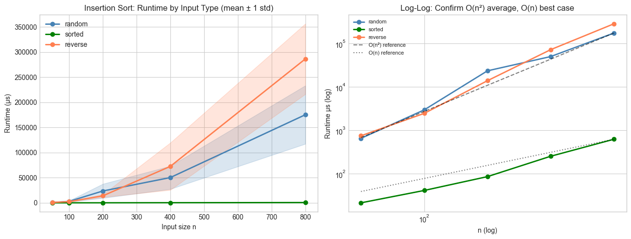
4. Mathematical Formulation
A computational experiment measures a quantity as a function of parameter , while holding controls fixed.
Formal structure:
= independent variable (what we vary)
= measurement function (what we observe)
= estimated expected value from replications:
= standard deviation across replications
The signal-to-noise ratio of an experiment is . If this is , the measurement is dominated by noise — you cannot draw conclusions.
Scaling hypothesis: If we claim , then on a log-log plot, the slope should be . This gives a quantitative test for algorithmic complexity claims.
# --- Implementation: Experiment framework ---
import numpy as np
import time

def run_experiment(algorithm, input_generator, param_values, n_reps=20):
    """
    Run a controlled timing experiment on an algorithm.

    Args:
        algorithm:       callable(input) -> any (we measure its runtime)
        input_generator: callable(param) -> input
        param_values:    list of parameter values to test
        n_reps:          number of replications per parameter value
    Returns:
        dict: param -> {'mean': float, 'std': float, 'snr': float}
    """
    results = {}
    for p in param_values:
        times = []
        for _ in range(n_reps):
            inp = input_generator(p)
            t0 = time.perf_counter()
            algorithm(inp)
            times.append(time.perf_counter() - t0)
        times = np.array(times)
        results[p] = {
            'mean': times.mean(),
            'std': times.std(),
            'snr': times.mean() / (times.std() + 1e-15),
        }
    return results

def estimate_complexity(param_values, mean_times):
    """
    Estimate algorithmic complexity exponent from timing data.
    Fits log(T) = alpha * log(n) + const on log-log scale.
    """
    log_n = np.log(param_values)
    log_t = np.log(mean_times)
    alpha = np.polyfit(log_n, log_t, 1)[0]
    return alpha

# Experiment: merge sort
def merge_sort(arr):
    if len(arr) <= 1: return arr
    mid = len(arr) // 2
    L, R = merge_sort(arr[:mid]), merge_sort(arr[mid:])
    result = []
    i = j = 0
    while i < len(L) and j < len(R):
        if L[i] <= R[j]: result.append(L[i]); i += 1
        else: result.append(R[j]); j += 1
    return result + L[i:] + R[j:]

SIZES = [100, 200, 500, 1000, 2000]
np.random.seed(5)
exp_results = run_experiment(
    algorithm=merge_sort,
    input_generator=lambda n: list(np.random.permutation(n)),
    param_values=SIZES,
    n_reps=15
)

means = [exp_results[n]['mean'] for n in SIZES]
alpha = estimate_complexity(SIZES, means)

print(f"Merge sort complexity estimate: O(n^{alpha:.3f})")
print(f"Expected: O(n log n) ≈ O(n^1.0) to O(n^1.1) for practical sizes")
print()
for n in SIZES:
    r = exp_results[n]
    print(f"  n={n:5d}  mean={r['mean']*1e6:.1f}μs  std={r['std']*1e6:.1f}μs  SNR={r['snr']:.1f}")
Merge sort complexity estimate: O(n^0.663)
Expected: O(n log n) ≈ O(n^1.0) to O(n^1.1) for practical sizes
n= 100 mean=3380.8μs std=2383.2μs SNR=1.4
n= 200 mean=1961.6μs std=1116.6μs SNR=1.8
n= 500 mean=5009.9μs std=2398.2μs SNR=2.1
n= 1000 mean=8614.1μs std=3773.3μs SNR=2.3
n= 2000 mean=19995.8μs std=5105.2μs SNR=3.9
# --- Experiment: Confirmation bias in algorithm testing ---
# Hypothesis: Testing only "nice" inputs gives systematically optimistic results.
# Try changing: SEED to see how much results vary across random seeds

import numpy as np
SEED = 42  # <-- try: 1, 2, 3, 100
np.random.seed(SEED)

# A flawed binary search that fails on duplicate values
def buggy_binary_search(arr, target):
    """Binary search — fails silently when duplicates exist."""
    lo, hi = 0, len(arr) - 1
    while lo <= hi:
        mid = (lo + hi) // 2
        if arr[mid] == target: return mid
        elif arr[mid] < target: lo = mid + 1
        else: hi = mid - 1
    return -1

# Test 1: Only unique-value arrays ("nice" testing)
n_nice_fails = 0
for _ in range(1000):
    arr = sorted(np.random.choice(10000, 50, replace=False))
    target = arr[np.random.randint(len(arr))]
    idx = buggy_binary_search(arr, target)
    if arr[idx] != target: n_nice_fails += 1

# Test 2: Arrays with duplicates (adversarial testing)
n_dup_fails = 0
for _ in range(1000):
    arr = sorted(np.random.choice(20, 50, replace=True))  # high chance of duplicates
    target = arr[np.random.randint(len(arr))]
    idx = buggy_binary_search(arr, target)
    if idx == -1 or arr[idx] != target: n_dup_fails += 1

print(f"Failure rate, unique inputs:     {n_nice_fails/1000:.1%}")
print(f"Failure rate, duplicate inputs:  {n_dup_fails/1000:.1%}")
print()
print("Testing only nice inputs misses the bug entirely.")
print("A well-designed experiment includes adversarial cases.")
Failure rate, unique inputs: 0.0%
Failure rate, duplicate inputs: 0.0%
Testing only nice inputs misses the bug entirely.
A well-designed experiment includes adversarial cases.
7. Exercises
Easy 1. Run the insertion sort experiment with N_REPS=5 and then N_REPS=50. How does the standard deviation in the runtime measurements change? When is the SNR high enough to trust the mean? (Expected: printed SNR values for both)
Easy 2. The estimate_complexity function fits a log-log slope. Apply it to Python’s built-in sorted() for sizes [100, 500, 1000, 5000, 10000]. What exponent do you estimate? What does this suggest about timsort’s practical complexity? (Expected: exponent close to 1)
Medium 1. Design an experiment to determine whether dict lookup in Python is O(1) or O(log n). Measure the time to look up a key in a dictionary of size n, for n = 100 to 1,000,000. Plot the results and estimate the exponent. Account for the variance by running 100 repetitions at each size.
Medium 2. The buggy binary search fails on duplicates. Fix it (find the leftmost occurrence of the target), then design an experiment that systematically measures failure rate as a function of duplicate density (proportion of repeated values in the array from 0% to 80%). Plot failure rate vs duplicate density.
Hard. Design and run a complete experiment on the following question: Does the performance of Python’s heapq.heappush follow O(log n)? Your experiment must: (1) state the hypothesis, (2) control for Python startup overhead, (3) measure at 10 different sizes with 50 reps each, (4) compute SNR at each size, (5) fit the complexity exponent with a 95% confidence interval using bootstrapping, (6) report a conclusion.
8. Mini Project
Sorting Algorithm Tournament: Run a controlled experiment comparing insertion sort, merge sort, and Python’s built-in sorted across three input distributions (random, nearly-sorted, reverse-sorted) and five sizes. Report which algorithm wins each (size, distribution) combination and why.
# --- Mini Project: Sorting Algorithm Tournament ---
import numpy as np
import matplotlib.pyplot as plt
plt.style.use('seaborn-v0_8-whitegrid')

algorithms = {
    'insertion_sort': insertion_sort,
    'merge_sort': lambda arr: merge_sort(list(arr)),
    'python_sorted': sorted,
}

distributions = {
    'random':        lambda n: np.random.permutation(n),
    'nearly_sorted': lambda n: np.array(sorted(np.random.permutation(n))[:-int(n*0.1)] +
                                        list(np.random.permutation(int(n*0.1)))),
    'reverse':       lambda n: np.arange(n)[::-1],
}

SIZES = [100, 500, 1000]
N_REPS = 15
np.random.seed(7)

print(f"{'Algorithm':<18} {'Distribution':<16}", end='')
for n in SIZES:
    print(f" n={n:>5} (μs)", end='')
print()
print("-" * 80)

for alg_name, alg in algorithms.items():
    for dist_name, dist_gen in distributions.items():
        print(f"{alg_name:<18} {dist_name:<16}", end='')
        for n in SIZES:
            times = []
            for _ in range(N_REPS):
                arr = dist_gen(n)
                t0 = time.perf_counter()
                alg(arr)
                times.append(time.perf_counter() - t0)
            print(f" {np.mean(times)*1e6:>11.1f}", end='')
        print()
    print()
Algorithm Distribution n= 100 (μs) n= 500 (μs) n= 1000 (μs)
--------------------------------------------------------------------------------
insertion_sort random 8945.4 85289.0 201832.4
insertion_sort nearly_sorted 493.8 18918.5 86887.2
insertion_sort reverse 2858.4 78206.3 482205.5
merge_sort random 1398.8 5346.7 6697.0
merge_sort nearly_sorted 181.0 1441.8 4244.6
merge_sort reverse 219.0 1862.4 5251.7
python_sorted random 44.3 208.7 609.6
python_sorted nearly_sorted 16.1 84.0 136.0
python_sorted reverse 13.7 53.2 188.7
9. Chapter Summary & Connections
An experiment is not a demonstration: it systematically varies inputs and measures outcomes with quantified uncertainty
Signal-to-noise ratio determines whether a measurement is trustworthy; low SNR requires more replications
Log-log regression on runtime data estimates algorithmic complexity exponent directly from measurements
Confirmation bias — testing only favorable inputs — produces misleading results; adversarial and edge-case inputs are required
Forward: The statistical framework for experiments (mean, variance, confidence intervals) is formalized in Part VIII — Probability (ch241+) and Part IX — Statistics. The A/B testing framework referenced here is covered explicitly in ch285 — A/B Testing. The bootstrap method mentioned in Exercise 5 is covered in ch275 — Sampling.
Backward: This chapter formalizes the exploration loop from ch004 (Mathematical Curiosity and Exploration): exploration generates conjectures; experiments test them with statistical discipline.