Prerequisites: ch001-ch017
You will learn:
A systematic method for converting an ambiguous real-world problem into a precise mathematical formulation
How to identify which mathematical structure fits a problem before solving it
How to communicate a model’s assumptions and limitations
Three case studies in different domains
Environment: Python 3.x, numpy, matplotlib
1. Concept
Most real-world problems are stated in natural language and are ambiguous. Mathematics requires precision. The translation step is where most modeling errors occur.
The translation checklist:
What is the unknown? Identify what is being predicted or optimized. Assign it a symbol and type.
What are the inputs? List all given or observable quantities. Assign symbols. Note units.
What are the constraints? What must be true? These become equations or inequalities.
What is the objective? Minimize error? Maximize profit? Find a root? This determines the tool.
What are the assumptions? List everything assumed but not guaranteed. These are the model’s limits.
What is the mathematical structure? Linear system? Optimization? Differential equation? Probability model?
Common misconception: A more complex problem requires a more complex model.
Sometimes the right move is to find a simpler problem that approximates the real one. Identifying the dominant effect and modeling only that is often more valuable.
2. Intuition & Mental Models
Physical analogy: Medical diagnosis. A physician clarifies the complaint (unknown?), takes measurements (inputs?), applies diagnostic criteria (constraints?), and forms a differential diagnosis (structures?). The translation checklist is the diagnostic protocol for mathematical problems.
Computational analogy: Requirements engineering. Converting “I want something that handles payments” into precise technical specifications (API, data models, SLAs) is the same translation process.
Recall from ch017 (Mathematical Modeling): we built the validation loop. This chapter focuses on getting the formulation right before attempting any solution.
# --- Visualization: Three case studies ---
import numpy as np
import matplotlib.pyplot as plt
plt.style.use('seaborn-v0_8-whitegrid')

fig, axes = plt.subplots(1, 3, figsize=(15, 5))

# Case 1: Optimal pricing
prices = np.linspace(0, 100, 300)
demand = np.maximum(1000 - 8*prices, 0)
revenue = prices * demand
opt_price = prices[np.argmax(revenue)]
axes[0].plot(prices, revenue/1000, 'steelblue', lw=2)
axes[0].axvline(opt_price, color='red', linestyle='--', label=f'Optimal ${opt_price:.0f}')
axes[0].set_xlabel('Price ($)'); axes[0].set_ylabel('Revenue ($1000s)')
axes[0].set_title('Case 1: Optimal Pricing\nRevenue = price x demand(price)')
axes[0].legend()

# Case 2: Minimum path through river crossing
A = np.array([0.0, 0.0]); B = np.array([5.0, 3.0]); RIVER_Y = 1.0
xs = np.linspace(0, 5, 300)
lengths = np.sqrt(xs**2 + RIVER_Y**2) + np.sqrt((5-xs)**2 + (3-RIVER_Y)**2)
opt_x = xs[np.argmin(lengths)]
axes[1].set_xlim(-0.5, 5.5); axes[1].set_ylim(-0.3, 3.5)
axes[1].axhline(RIVER_Y, color='cyan', lw=4, alpha=0.5, label='River bank')
axes[1].plot(*A, 'ko', markersize=10, label='A'); axes[1].plot(*B, 'rs', markersize=10, label='B')
axes[1].plot([A[0], opt_x, B[0]], [A[1], RIVER_Y, B[1]], 'g-o', lw=2, label=f'x={opt_x:.2f}')
axes[1].set_title(f'Case 2: Shortest Cable Path\nMin length = {lengths.min():.3f}')
axes[1].set_xlabel('x'); axes[1].set_ylabel('y'); axes[1].legend(fontsize=8)

# Case 3: EOQ
DEMAND_ANNUAL, ORDER_COST, HOLDING_COST = 1000, 50, 2
qs = np.linspace(10, 500, 300)
total_cost = (DEMAND_ANNUAL/qs)*ORDER_COST + (qs/2)*HOLDING_COST
EOQ = np.sqrt(2*DEMAND_ANNUAL*ORDER_COST/HOLDING_COST)
axes[2].plot(qs, (DEMAND_ANNUAL/qs)*ORDER_COST, '--', label='Ordering cost', alpha=0.7)
axes[2].plot(qs, (qs/2)*HOLDING_COST, ':', label='Holding cost', alpha=0.7)
axes[2].plot(qs, total_cost, 'steelblue', lw=2, label='Total cost')
axes[2].axvline(EOQ, color='red', linestyle='--', label=f'EOQ={EOQ:.0f}')
axes[2].set_xlabel('Order qty'); axes[2].set_ylabel('Annual cost ($)')
axes[2].set_title(f'Case 3: Inventory (EOQ)\nEOQ = sqrt(2DS/H) = {EOQ:.0f}')
axes[2].legend(fontsize=8); axes[2].set_ylim(0, 2000)
plt.tight_layout(); plt.show()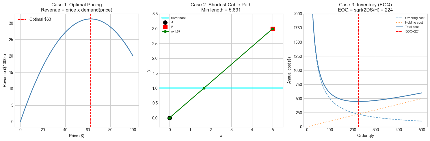
4. Mathematical Formulation
Three canonical structures encountered here:
Optimization: maximize f(x) subject to g(x) <= 0. Solved by f’(x) = 0.
Geometric path: minimize distance d(P,Q) = ||P-Q|| over feasible set. Optimize over a parameter.
Cost-balancing (EOQ): C(q) = (D/q)*S + (q/2)H. Differentiate: dC/dq = 0 gives q = sqrt(2DS/H).
The model structures differ; the solution method (zero of derivative) is the same. Recognizing the structure identifies the tool.
# --- Implementation: Problem formulation record ---
import numpy as np

class ProblemFormulation:
    def __init__(self, problem_statement):
        self.problem = problem_statement
        self.unknowns = {}; self.inputs = {}
        self.constraints = []; self.objective = None
        self.assumptions = []; self.structure = None

    def add_unknown(self, symbol, description, domain):
        self.unknowns[symbol] = {'description': description, 'domain': domain}; return self
    def add_input(self, symbol, description, value=None):
        self.inputs[symbol] = {'description': description, 'value': value}; return self
    def add_constraint(self, expression, description):
        self.constraints.append({'expr': expression, 'desc': description}); return self
    def set_objective(self, description, fn=None):
        self.objective = {'description': description, 'fn': fn}; return self
    def add_assumption(self, text):
        self.assumptions.append(text); return self
    def set_structure(self, s):
        self.structure = s; return self

    def report(self):
        print(f"PROBLEM: {self.problem}")
        print(f"Unknown: {self.unknowns}")
        print(f"Inputs:  {[(s, d['value']) for s,d in self.inputs.items()]}")
        print(f"Constraints: {[c['expr'] for c in self.constraints]}")
        print(f"Objective: {self.objective['description'] if self.objective else 'unset'}")
        print(f"Assumptions: {self.assumptions}")
        print(f"Structure: {self.structure}")

# Formalize the EOQ problem
eoq = ProblemFormulation("Minimize annual inventory cost")
eoq.add_unknown('q', 'Order quantity per order', 'positive reals')
eoq.add_input('D', 'Annual demand (units/year)', 1000)
eoq.add_input('S', 'Order cost per order ($)', 50)
eoq.add_input('H', 'Holding cost per unit per year ($)', 2)
eoq.add_constraint('q > 0', 'Cannot order negative quantity')
eoq.set_objective('Minimize C(q) = (D/q)*S + (q/2)*H')
eoq.add_assumption('Demand is constant throughout the year')
eoq.add_assumption('Lead time is zero -- instantaneous delivery')
eoq.set_structure('Univariate calculus optimization: dC/dq = 0')
eoq.report()

D, S, H = 1000, 50, 2
EOQ = (2*D*S/H)**0.5
print(f"\nSolution: q* = sqrt(2DS/H) = {EOQ:.2f} units")
PROBLEM: Minimize annual inventory cost
Unknown: {'q': {'description': 'Order quantity per order', 'domain': 'positive reals'}}
Inputs: [('D', 1000), ('S', 50), ('H', 2)]
Constraints: ['q > 0']
Objective: Minimize C(q) = (D/q)*S + (q/2)*H
Assumptions: ['Demand is constant throughout the year', 'Lead time is zero -- instantaneous delivery']
Structure: Univariate calculus optimization: dC/dq = 0
Solution: q* = sqrt(2DS/H) = 223.61 units
# --- Experiment: Sensitivity of EOQ to input errors ---
import numpy as np
import matplotlib.pyplot as plt
plt.style.use('seaborn-v0_8-whitegrid')

ERROR = 0.20  # try: 0.05, 0.50
D_true, S_true, H_true = 1000, 50, 2
EOQ_true = (2*D_true*S_true/H_true)**0.5
np.random.seed(42)
N = 1000
D_obs = D_true * (1 + ERROR*np.random.randn(N))
S_obs = S_true * (1 + ERROR*np.random.randn(N))
H_obs = np.maximum(H_true * (1 + ERROR*np.random.randn(N)), 0.01)
EOQ_obs = (2*D_obs*S_obs/H_obs)**0.5
rel_err = (EOQ_obs - EOQ_true) / EOQ_true

fig, ax = plt.subplots(figsize=(9, 4))
ax.hist(rel_err*100, bins=40, alpha=0.7, edgecolor='white')
ax.axvline(0, color='red', lw=2, linestyle='--')
ax.set_xlabel('Relative error in EOQ (%)')
ax.set_title(f'EOQ Sensitivity to {ERROR*100:.0f}% Input Errors (output std: {rel_err.std()*100:.1f}%)')
plt.tight_layout(); plt.show()
print("EOQ is robust: output error approximately equals input error / 2")
print("This is a known property -- the cost function is flat near the optimum.")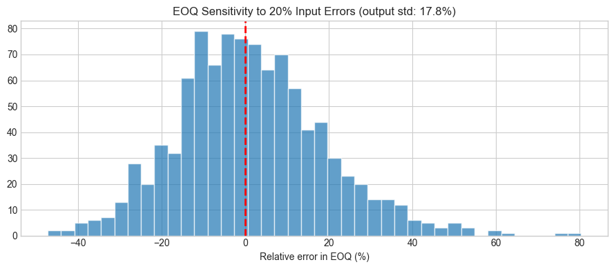
EOQ is robust: output error approximately equals input error / 2
This is a known property -- the cost function is flat near the optimum.
7. Exercises
Easy 1. Formulate using ProblemFormulation: A farmer has 100m of fencing against a barn wall (3 sides needed). Maximize enclosed area. Solve analytically (derivative) and verify numerically.
Easy 2. For Case 1 with exponential demand D(p) = 1000 * e^(-0.05p), find the optimal price numerically using grid search on [0, 100].
Medium 1. Cable problem generalization: cost per unit length is c1 on land, c2 underwater. Find optimal crossing for c2/c1 in {1.0, 2.0, 5.0}.
Medium 2. Formulate: CPU has 3 tasks with deadlines. Task A: 5ms exec, 10ms deadline. Task B: 3ms exec, 7ms deadline. Task C: 4ms exec, 12ms deadline. What order minimizes missed deadlines? What mathematical structure is this?
Hard. Model the herd immunity threshold: given basic reproduction number R0, what vaccination fraction v* prevents epidemic spread? Derive v* = 1 - 1/R0. Verify with SIR simulation for R0 in {1.5, 2.0, 3.0, 5.0}.
# --- Mini Project: Formulation pipeline ---
ad_problem = ProblemFormulation("Maximize profit from online advertising campaign")
ad_problem.add_unknown('b', 'Daily budget ($)', 'positive reals')
ad_problem.add_input('CPC', 'Cost per click ($)', 0.50)
ad_problem.add_input('CVR', 'Conversion rate', 0.03)
ad_problem.add_input('AOV', 'Average order value ($)', 45.00)
ad_problem.add_input('COGS', 'Cost of goods sold ($)', 20.00)
ad_problem.set_objective('Maximize profit = b * (CVR/CPC * (AOV-COGS) - 1)')
ad_problem.add_assumption('Click volume is proportional to spend (linear response)')
ad_problem.add_assumption('Conversion rate is constant -- no diminishing returns')
ad_problem.set_structure('Linear objective: spend until budget cap or until ROI < 1')
ad_problem.report()

CPC, CVR, AOV, COGS = 0.50, 0.03, 45.0, 20.0
profit_per_dollar = CVR/CPC*(AOV-COGS) - 1
print(f"\nProfit per $ spent: {profit_per_dollar:.4f}")
print("Campaign is profitable -- spend to budget limit." if profit_per_dollar > 0
      else "Campaign is unprofitable -- do not spend.")
PROBLEM: Maximize profit from online advertising campaign
Unknown: {'b': {'description': 'Daily budget ($)', 'domain': 'positive reals'}}
Inputs: [('CPC', 0.5), ('CVR', 0.03), ('AOV', 45.0), ('COGS', 20.0)]
Constraints: []
Objective: Maximize profit = b * (CVR/CPC * (AOV-COGS) - 1)
Assumptions: ['Click volume is proportional to spend (linear response)', 'Conversion rate is constant -- no diminishing returns']
Structure: Linear objective: spend until budget cap or until ROI < 1
Profit per $ spent: 0.5000
Campaign is profitable -- spend to budget limit.
9. Chapter Summary & Connections
The six-step translation checklist (unknown, inputs, constraints, objective, assumptions, structure) converts ambiguous real problems to precise mathematics
Structure identification is the key step: it connects the specific problem to a class with known solution methods
The EOQ model is robust: its solution is insensitive to moderate input errors because the cost function is flat near the optimum
Sensitivity analysis is a required part of any model delivered to a decision-maker
Forward: The three canonical structures here (optimization, path, cost-balancing) are unified in ch201 -- Why Calculus Matters, where all three are solved by finding where the derivative is zero. Sensitivity analysis is formalized in ch211 -- Partial Derivatives.
Backward: Applies every tool from Part I: modeling cycle from ch017, assumption tracking, structure identification from ch003, visualization from ch008.