Chapter 20 -- Part I Capstone Project
Concepts used from this Part:
ch001: Mathematical curiosity, self-diagnostic tools
ch003: Abstraction, modeling pipeline, structure identification
ch004: Exploration loop, conjecture testing
ch007: Computational experiments, property-based testing
ch008: Visualization as a learning tool
ch009/ch010: Mathematical notation, expression parsing
ch011/ch012: Set theory, Boolean algebra
ch015/ch016: Proof intuition, counterexample finding
ch019: Specification-first mathematical programming
Expected output: A working interactive tool for exploring mathematical expressions
Difficulty: Medium-Hard | Estimated time: 3-5 hours
0. Overview
Problem statement:
A symbolic math playground is a software environment for exploring mathematical expressions: evaluating them, plotting them, testing properties, finding patterns, and checking conjectures. Think of it as a lightweight, programmable calculator with mathematical awareness -- it knows what an expression means, not just what number it produces.
You will build this incrementally across five stages:
Expression library -- a collection of mathematical functions with full specification
Property tester -- tests algebraic identities on any collection of functions
Structure identifier -- identifies the mathematical structure of data
Conjecture engine -- generates, tests, and records mathematical conjectures
Visualization dashboard -- brings it all together in a unified visual interface
By the end, you will have a tool you can use throughout the rest of this book to explore new concepts before they are formally introduced.
What mathematics makes it possible:
Computational representation of functions (ch051+, anticipated here)
Property-based testing via logical quantifiers (ch012-ch013)
Structure identification via regression and log-log analysis (ch003, ch008)
Conjecture generation via numerical pattern detection (ch004)
Visualization via matplotlib (ch008)
1. Setup
# --- Setup: Imports, constants, base infrastructure ---
import numpy as np
import matplotlib.pyplot as plt
import matplotlib.gridspec as gridspec
from fractions import Fraction
import math
import random
from itertools import product as iproduct

plt.style.use('seaborn-v0_8-whitegrid')
np.random.seed(42)
random.seed(42)

# Approved function environment for safe eval
SAFE_ENV = {
    'sin': np.sin, 'cos': np.cos, 'tan': np.tan,
    'exp': np.exp, 'log': np.log, 'log2': np.log2, 'log10': np.log10,
    'sqrt': np.sqrt, 'abs': np.abs,
    'pi': np.pi, 'e': np.e,
    'floor': np.floor, 'ceil': np.ceil,
    'sign': np.sign,
}

print("Symbolic Math Playground -- initializing...")
print(f"Available functions: {sorted(SAFE_ENV.keys())}")
print("Ready.")
Symbolic Math Playground -- initializing...
Available functions: ['abs', 'ceil', 'cos', 'e', 'exp', 'floor', 'log', 'log10', 'log2', 'pi', 'sign', 'sin', 'sqrt', 'tan']
Ready.
2. Stage 1 -- Expression Library
Build a MathExpression class that wraps a string formula and provides: evaluation, differentiation (numerical), integration (numerical), and domain detection.
# --- Stage 1: MathExpression class ---
# Each expression is fully specified: formula, domain, properties.

class MathExpression:
    """
    A mathematical expression with specification, evaluation, and analysis.

    Specification:
        Input:  formula string with variable 'x'
        Domain: interval [a, b] where formula is defined and real-valued
        Output: float value or array
    """
    def __init__(self, formula, domain=(-10, 10), name=None):
        self.formula = formula
        self.domain = domain
        self.name = name or formula
        self._validate_domain()

    def _validate_domain(self):
        """Check that the formula evaluates without error in the domain."""
        x = np.linspace(self.domain[0], self.domain[1], 20)
        try:
            result = eval(self.formula, {'x': x, **SAFE_ENV})
            if not np.all(np.isfinite(result)):
                raise ValueError(f"Formula produces non-finite values in domain")
        except Exception as e:
            raise ValueError(f"Formula validation failed: {e}")

    def evaluate(self, x):
        """Evaluate the expression at scalar or array x."""
        x = np.asarray(x, dtype=float)
        return eval(self.formula, {'x': x, **SAFE_ENV})

    def derivative(self, x, h=1e-6):
        """Numerical derivative using central difference."""
        return (self.evaluate(x + h) - self.evaluate(x - h)) / (2 * h)

    def integrate(self, a=None, b=None, n=10000):
        """Numerical integral using trapezoidal rule."""
        a = a or self.domain[0]
        b = b or self.domain[1]
        x = np.linspace(a, b, n)
        return np.trapezoid(self.evaluate(x), x)

    def sample_points(self, n=200):
        """Return evenly spaced (x, f(x)) pairs in the domain."""
        x = np.linspace(self.domain[0], self.domain[1], n)
        return x, self.evaluate(x)

    def plot(self, ax=None, **kwargs):
        """Plot the expression on its domain."""
        if ax is None:
            fig, ax = plt.subplots(figsize=(8, 4))
        x, y = self.sample_points()
        ax.plot(x, y, label=self.name, **kwargs)
        ax.set_xlabel('x'); ax.set_ylabel('f(x)')
        ax.set_title(f'f(x) = {self.name}')
        return ax

    def __repr__(self):
        return f"MathExpression('{self.formula}', domain={self.domain})"

# Build the expression library
LIBRARY = {
    'linear':      MathExpression('2*x + 3',             (-5, 5),    'linear: 2x+3'),
    'quadratic':   MathExpression('x**2 - 2*x + 1',      (-3, 5),    'quadratic: (x-1)^2'),
    'cubic':       MathExpression('x**3 - 3*x',          (-2.5, 2.5),'cubic: x^3-3x'),
    'sine':        MathExpression('sin(x)',               (-2*np.pi, 2*np.pi), 'sin(x)'),
    'damped_sine': MathExpression('sin(x) * exp(-0.2*x)', (0, 4*np.pi), 'sin(x)*exp(-0.2x)'),
    'sigmoid':     MathExpression('1 / (1 + exp(-x))',   (-6, 6),    'sigmoid: 1/(1+e^-x)'),
    'gaussian':    MathExpression('exp(-x**2 / 2)',      (-4, 4),    'Gaussian: e^(-x^2/2)'),
    'log_growth':  MathExpression('log(x)',              (0.01, 10), 'log(x)'),
    'power_law':   MathExpression('x**1.5',              (0, 8),     'power: x^1.5'),
    'reciprocal':  MathExpression('1 / (1 + x**2)',      (-5, 5),    'Cauchy: 1/(1+x^2)'),
}

print(f"Expression library: {len(LIBRARY)} functions")
for name, expr in LIBRARY.items():
    a, b = expr.domain
    x_mid = (a + b) / 2
    print(f"  {name:<15}: f({x_mid:.1f}) = {expr.evaluate(x_mid):.4f}")
Expression library: 10 functions
linear : f(0.0) = 3.0000
quadratic : f(1.0) = 0.0000
cubic : f(0.0) = 0.0000
sine : f(0.0) = 0.0000
damped_sine : f(6.3) = -0.0000
sigmoid : f(0.0) = 0.5000
gaussian : f(0.0) = 1.0000
log_growth : f(5.0) = 1.6104
power_law : f(4.0) = 8.0000
reciprocal : f(0.0) = 1.0000
3. Stage 2 -- Property Tester
Build a system that tests algebraic properties of expressions: symmetry (even/odd), periodicity, monotonicity, and custom user-defined properties.
# --- Stage 2: Property tester ---

class PropertyTester:
    """
    Tests algebraic properties of MathExpression objects.
    Uses randomized testing over the expression's domain.
    """
    def __init__(self, expr, n_tests=500, tolerance=1e-6):
        self.expr = expr
        self.n_tests = n_tests
        self.tol = tolerance
        np.random.seed(0)

    def _random_points(self):
        a, b = self.expr.domain
        return np.random.uniform(a, b, self.n_tests)

    def test_even(self):
        """f is even iff f(x) == f(-x) for all x in domain."""
        a, b = self.expr.domain
        x = np.random.uniform(0, min(abs(a), abs(b)), self.n_tests)
        lhs = self.expr.evaluate(x)
        rhs = self.expr.evaluate(-x)
        return np.all(np.abs(lhs - rhs) < self.tol), np.max(np.abs(lhs - rhs))

    def test_odd(self):
        """f is odd iff f(-x) == -f(x) for all x."""
        a, b = self.expr.domain
        x = np.random.uniform(0, min(abs(a), abs(b)), self.n_tests)
        lhs = self.expr.evaluate(-x)
        rhs = -self.expr.evaluate(x)
        return np.all(np.abs(lhs - rhs) < self.tol), np.max(np.abs(lhs - rhs))

    def test_periodic(self, period):
        """f is periodic with period T iff f(x+T) == f(x) for all x."""
        a, b = self.expr.domain
        x = np.random.uniform(a, b - period, min(self.n_tests, 200))
        lhs = self.expr.evaluate(x)
        rhs = self.expr.evaluate(x + period)
        return np.all(np.abs(lhs - rhs) < self.tol), np.max(np.abs(lhs - rhs))

    def test_monotone_increasing(self):
        """f is monotone increasing iff f'(x) >= 0 for all x in domain."""
        x = self._random_points()
        deriv = self.expr.derivative(x)
        return np.all(deriv >= -self.tol), float(np.min(deriv))

    def test_nonnegative(self):
        """f(x) >= 0 for all x in domain."""
        x = self._random_points()
        vals = self.expr.evaluate(x)
        return np.all(vals >= -self.tol), float(np.min(vals))

    def full_report(self):
        results = {}
        results['even']       = self.test_even()
        results['odd']        = self.test_odd()
        results['periodic_2pi'] = self.test_periodic(2 * np.pi)
        results['monotone_increasing'] = self.test_monotone_increasing()
        results['nonnegative'] = self.test_nonnegative()

        print(f"Property report: {self.expr.name}")
        print(f"{'Property':<25} {'Holds':>7} {'Max deviation':>15}")
        print('-' * 50)
        for name, (holds, deviation) in results.items():
            print(f"  {name:<23} {'YES' if holds else 'no':>7} {deviation:>15.2e}")
        return results

# Test all library expressions
print("Running property tests on expression library...")
for key in ['sine', 'gaussian', 'quadratic', 'sigmoid', 'cubic']:
    tester = PropertyTester(LIBRARY[key])
    tester.full_report()
    print()
Running property tests on expression library...
Property report: sin(x)
Property Holds Max deviation
--------------------------------------------------
even no 2.00e+00
odd YES 0.00e+00
periodic_2pi YES 2.78e-16
monotone_increasing no -1.00e+00
nonnegative no -1.00e+00
Property report: Gaussian: e^(-x^2/2)
Property Holds Max deviation
--------------------------------------------------
even YES 0.00e+00
odd no 2.00e+00
periodic_2pi no 7.33e-02
monotone_increasing no -6.06e-01
nonnegative YES 3.36e-04
Property report: quadratic: (x-1)^2
Property Holds Max deviation
--------------------------------------------------
even no 1.20e+01
odd no 2.00e+01
periodic_2pi no 1.08e+01
monotone_increasing no -7.99e+00
nonnegative YES 4.39e-05
Property report: sigmoid: 1/(1+e^-x)
Property Holds Max deviation
--------------------------------------------------
even no 9.95e-01
odd no 1.00e+00
periodic_2pi no 9.17e-01
monotone_increasing YES 2.48e-03
nonnegative YES 2.47e-03
Property report: cubic: x^3-3x
Property Holds Max deviation
--------------------------------------------------
even no 1.62e+01
odd YES 0.00e+00
periodic_2pi no 5.09e+01
monotone_increasing no -3.00e+00
nonnegative no -8.12e+00
4. Stage 3 -- Structure Identifier
Given any dataset (t, y), identify which mathematical structure best describes it using the log-log regression technique from ch008.
# --- Stage 3: Structure identifier ---

class StructureIdentifier:
    """
    Given data (x, y), identifies the best-fitting mathematical structure
    from: linear, quadratic, exponential, logarithmic, power law.
    Uses linearization: each structure becomes linear under a transformation.
    """

    STRUCTURES = {
        'linear':      (lambda x,y: (x, y),           'y = ax + b'),
        'quadratic':   (lambda x,y: (x, y),           'y = ax^2+bx+c'),  # fit degree 2
        'exponential': (lambda x,y: (x, np.log(y)),   'y = a*exp(bx)'),
        'logarithmic': (lambda x,y: (np.log(x), y),   'y = a*log(x)+b'),
        'power_law':   (lambda x,y: (np.log(x), np.log(y)), 'y = a*x^b'),
    }

    def identify(self, x, y, verbose=True):
        x = np.array(x, dtype=float)
        y = np.array(y, dtype=float)
        valid = (x > 0) & (y > 0) & np.isfinite(x) & np.isfinite(y)

        scores = {}

        # Linear and quadratic: direct polynomial fit
        for degree, name in [(1, 'linear'), (2, 'quadratic')]:
            coeffs = np.polyfit(x, y, degree)
            y_pred = np.polyval(coeffs, x)
            ss_res = np.sum((y - y_pred)**2)
            ss_tot = np.sum((y - y.mean())**2)
            scores[name] = 1 - ss_res/ss_tot if ss_tot > 0 else 0

        # Linearizable structures
        if valid.sum() > 3:
            xv, yv = x[valid], y[valid]
            for name in ['exponential', 'logarithmic', 'power_law']:
                transform, _ = self.STRUCTURES[name]
                xt, yt = transform(xv, yv)
                if np.all(np.isfinite(xt)) and np.all(np.isfinite(yt)):
                    coeffs = np.polyfit(xt, yt, 1)
                    yt_pred = np.polyval(coeffs, xt)
                    ss_res = np.sum((yv - np.exp(yt_pred) if 'exp' in name or 'power' in name
                                     else yv - yt_pred)**2)
                    ss_tot = np.sum((yv - yv.mean())**2)
                    scores[name] = 1 - ss_res/ss_tot if ss_tot > 0 else 0

        best = max(scores, key=lambda k: scores[k])
        if verbose:
            print(f"{'Structure':<15} {'R2':>8}")
            print('-' * 26)
            for s in sorted(scores, key=lambda k: -scores[k]):
                marker = ' <-- BEST' if s == best else ''
                print(f"  {s:<13} {scores[s]:>8.4f}{marker}")
            _, desc = self.STRUCTURES[best]
            print(f"\nIdentified structure: {desc}")
        return best, scores

identifier = StructureIdentifier()
np.random.seed(3)
t = np.linspace(1, 20, 30)
noise = lambda: 0.03 * np.random.randn(len(t))

print("=== Test: power law data ===")
identifier.identify(t, 3.0 * t**2.1 * (1 + noise()))
print()
print("=== Test: exponential data ===")
identifier.identify(t, 5.0 * np.exp(0.15*t) * (1 + noise()))
print()
print("=== Test: logarithmic data ===")
identifier.identify(t, 8.0 * np.log(t) + 2 + 0.3*np.random.randn(len(t)))
=== Test: power law data ===
Structure R2
--------------------------
power_law 0.9989 <-- BEST
quadratic 0.9989
linear 0.9363
logarithmic 0.6842
exponential 0.2209
Identified structure: y = a*x^b
=== Test: exponential data ===
Structure R2
--------------------------
exponential 0.9961 <-- BEST
quadratic 0.9954
linear 0.8903
power_law 0.7846
logarithmic 0.6215
Identified structure: y = a*exp(bx)
=== Test: logarithmic data ===
Structure R2
--------------------------
logarithmic 0.9974 <-- BEST
quadratic 0.9749
power_law 0.8821
linear 0.8660
exponential 0.6185
Identified structure: y = a*log(x)+b
('logarithmic',
 {'linear': np.float64(0.8660267574115534),
  'quadratic': np.float64(0.974903465063021),
  'exponential': np.float64(0.6185495360757487),
  'logarithmic': np.float64(0.9973572503683723),
  'power_law': np.float64(0.8820599459561225)})
5. Stage 4 -- Conjecture Engine
Build a system that automatically generates mathematical conjectures about expressions, tests them, and records the results in a structured log.
# --- Stage 4: Conjecture engine ---
class ConjectureEngine:
"""
Generates and tests mathematical conjectures about expressions.
Records all results in a structured log.
"""
def __init__(self):
self.conjectures = []
self.proven = []
self.refuted = []
def add_conjecture(self, name, predicate, domain, description):
"""
Register a conjecture for testing.
Args:
name: short identifier
predicate: callable(x) -> bool, the claim to test
domain: iterable of test values
description: precise statement of the claim
"""
self.conjectures.append({
'name': name, 'predicate': predicate,
'domain': domain, 'description': description,
})
def test_all(self, verbose=True):
"""Test all registered conjectures."""
for c in self.conjectures:
counterexample = None
tested = 0
for x in c['domain']:
tested += 1
try:
if not c['predicate'](x):
counterexample = x
break
except:
counterexample = x
break
result = {**c, 'tested': tested, 'counterexample': counterexample,
'holds': counterexample is None}
if counterexample is None:
self.proven.append(result)
else:
self.refuted.append(result)
if verbose:
status = 'CONSISTENT' if counterexample is None else 'REFUTED'
print(f" [{status}] {c['name']}: {c['description'][:60]}")
if counterexample is not None:
print(f" Counterexample: x = {counterexample:.4f}")
print(f"\nSummary: {len(self.proven)} consistent, {len(self.refuted)} refuted")
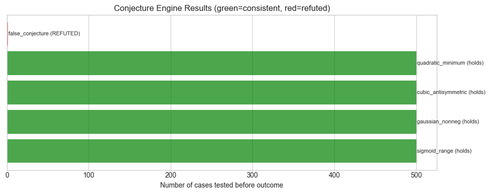
def summary_plot(self):
fig, ax = plt.subplots(figsize=(10, 4))
all_results = [(r, 'green') for r in self.proven] + [(r, 'red') for r in self.refuted]
for i, (r, color) in enumerate(all_results):
ax.barh(i, r['tested'], color=color, alpha=0.7)
label = r['name'] + (' (holds)' if r['holds'] else ' (REFUTED)')
ax.text(r['tested']+1, i, label, va='center', fontsize=8)
ax.set_xlabel('Number of cases tested before outcome')
ax.set_title('Conjecture Engine Results (green=consistent, red=refuted)')
ax.set_yticks([])
plt.tight_layout()
plt.show()
engine = ConjectureEngine()
# Register conjectures about our expression library
engine.add_conjecture(
'sigmoid_range',
lambda x: 0 < LIBRARY['sigmoid'].evaluate(x) < 1,
np.random.uniform(-6, 6, 500),
'sigmoid(x) is always in (0,1)'
)
engine.add_conjecture(
'gaussian_nonneg',
lambda x: LIBRARY['gaussian'].evaluate(x) >= 0,
np.random.uniform(-4, 4, 500),
'Gaussian exp(-x^2/2) >= 0 always'
)
engine.add_conjecture(
'cubic_antisymmetric',
lambda x: abs(LIBRARY['cubic'].evaluate(-x) + LIBRARY['cubic'].evaluate(x)) < 1e-9,
np.random.uniform(-2.4, 2.4, 500),
'x^3 - 3x is an odd function: f(-x) = -f(x)'
)
engine.add_conjecture(
'quadratic_minimum',
lambda x: LIBRARY['quadratic'].evaluate(x) >= 0,
np.random.uniform(-3, 5, 500),
'(x-1)^2 >= 0 always (perfect square nonnegative)'
)
engine.add_conjecture(
'false_conjecture',
lambda x: LIBRARY['cubic'].evaluate(x) > 0,
np.linspace(-2.4, 2.4, 200),
'x^3 - 3x > 0 always (FALSE -- negative for x in (-sqrt3, 0))'
)
print("Testing all conjectures...")
engine.test_all()
engine.summary_plot()Testing all conjectures...
[CONSISTENT] sigmoid_range: sigmoid(x) is always in (0,1)
[CONSISTENT] gaussian_nonneg: Gaussian exp(-x^2/2) >= 0 always
[CONSISTENT] cubic_antisymmetric: x^3 - 3x is an odd function: f(-x) = -f(x)
[CONSISTENT] quadratic_minimum: (x-1)^2 >= 0 always (perfect square nonnegative)
[REFUTED] false_conjecture: x^3 - 3x > 0 always (FALSE -- negative for x in (-sqrt3, 0))
Counterexample: x = -2.4000
Summary: 4 consistent, 1 refuted
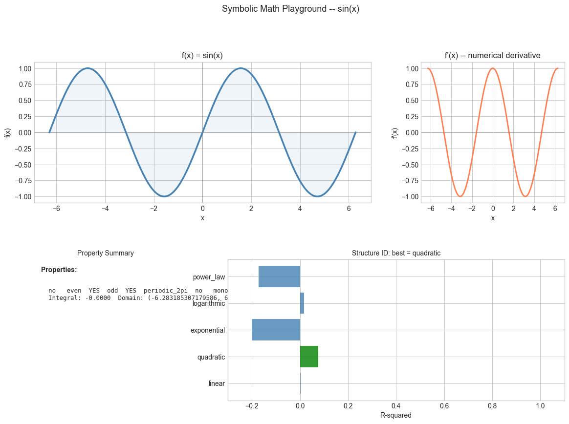
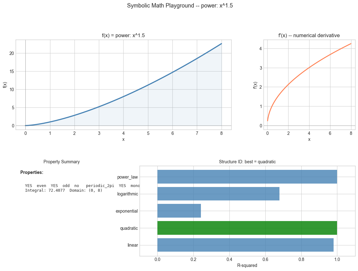
6. Stage 5 -- Visualization Dashboard
Bring all four stages together into a single visualization: plot the expression, annotate its properties, and show the structure identification result.
# --- Stage 5: Unified visualization dashboard ---

def math_dashboard(expr_name, structure_data=None):
    """
    Create a comprehensive visualization for one expression in the library.
    Shows: function plot, derivative, property summary, structure ID.
    """
    expr = LIBRARY[expr_name]
    tester = PropertyTester(expr)
    props = tester.full_report()

    fig = plt.figure(figsize=(14, 9))
    gs = gridspec.GridSpec(2, 3, figure=fig, hspace=0.4, wspace=0.35)

    # 1. Main function plot
    ax1 = fig.add_subplot(gs[0, :2])
    x, y = expr.sample_points(300)
    ax1.plot(x, y, 'steelblue', linewidth=2.5)
    ax1.axhline(0, color='gray', linewidth=0.8, alpha=0.5)
    ax1.axvline(0, color='gray', linewidth=0.8, alpha=0.5)
    ax1.set_title(f'f(x) = {expr.name}', fontsize=12)
    ax1.set_xlabel('x'); ax1.set_ylabel('f(x)')
    ax1.fill_between(x, 0, y, alpha=0.08, color='steelblue')

    # 2. Derivative
    ax2 = fig.add_subplot(gs[0, 2])
    deriv = expr.derivative(x)
    ax2.plot(x, deriv, 'coral', linewidth=2)
    ax2.axhline(0, color='gray', linewidth=0.8, alpha=0.5)
    ax2.set_title("f'(x) -- numerical derivative")
    ax2.set_xlabel('x'); ax2.set_ylabel("f'(x)")

    # 3. Property summary
    ax3 = fig.add_subplot(gs[1, 0])
    ax3.axis('off')
    prop_lines = []
    for pname, (holds, dev) in props.items():
        symbol = 'YES' if holds else 'no '
        prop_lines.append(f"  {symbol}  {pname}")

    integral_val = expr.integrate()
    prop_lines.append(f"\n  Integral: {integral_val:.4f}")
    prop_lines.append(f"  Domain: {expr.domain}")

    ax3.text(0.05, 0.95, 'Properties:', transform=ax3.transAxes,
             fontsize=10, fontweight='bold', verticalalignment='top')
    ax3.text(0.05, 0.80, ''.join(prop_lines), transform=ax3.transAxes,
             fontsize=9, verticalalignment='top', fontfamily='monospace')
    ax3.set_title('Property Summary', fontsize=10)

    # 4. Structure identification (if data provided)
    ax4 = fig.add_subplot(gs[1, 1:])
    if structure_data is not None:
        sx, sy = structure_data
        identifier_local = StructureIdentifier()
        best, scores = identifier_local.identify(sx, sy, verbose=False)

        names = list(scores.keys())
        vals = [scores[n] for n in names]
        colors = ['steelblue' if n != best else 'green' for n in names]
        ax4.barh(range(len(names)), vals, color=colors, alpha=0.8)
        ax4.set_yticks(range(len(names))); ax4.set_yticklabels(names)
        ax4.set_xlabel('R-squared')
        ax4.set_title(f'Structure ID: best = {best}', fontsize=10)
        ax4.set_xlim(min(0, min(vals)) - 0.1, 1.1)
    else:
        ax4.text(0.5, 0.5, 'No data provided forstructure identification',
                 ha='center', va='center', transform=ax4.transAxes, fontsize=10)
        ax4.axis('off')

    plt.suptitle(f'Symbolic Math Playground -- {expr.name}', fontsize=13, y=1.01)
    plt.tight_layout()
    plt.show()

# Run the dashboard for several expressions
for expr_name in ['sine', 'gaussian', 'sigmoid', 'power_law']:
    # Generate sample data from the expression + noise for structure ID
    expr = LIBRARY[expr_name]
    a, b = expr.domain
    t_sample = np.linspace(max(a, 0.1), b, 40)
    y_sample = expr.evaluate(t_sample) + 0.05 * np.random.randn(len(t_sample))
    math_dashboard(expr_name, structure_data=(t_sample, np.abs(y_sample)+0.001))
    print()
Property report: sin(x)
Property Holds Max deviation
--------------------------------------------------
even no 2.00e+00
odd YES 0.00e+00
periodic_2pi YES 2.78e-16
monotone_increasing no -1.00e+00
nonnegative no -1.00e+00
C:\Users\user\AppData\Local\Temp\ipykernel_24988\378153234.py:72: UserWarning: This figure includes Axes that are not compatible with tight_layout, so results might be incorrect.
  plt.tight_layout()
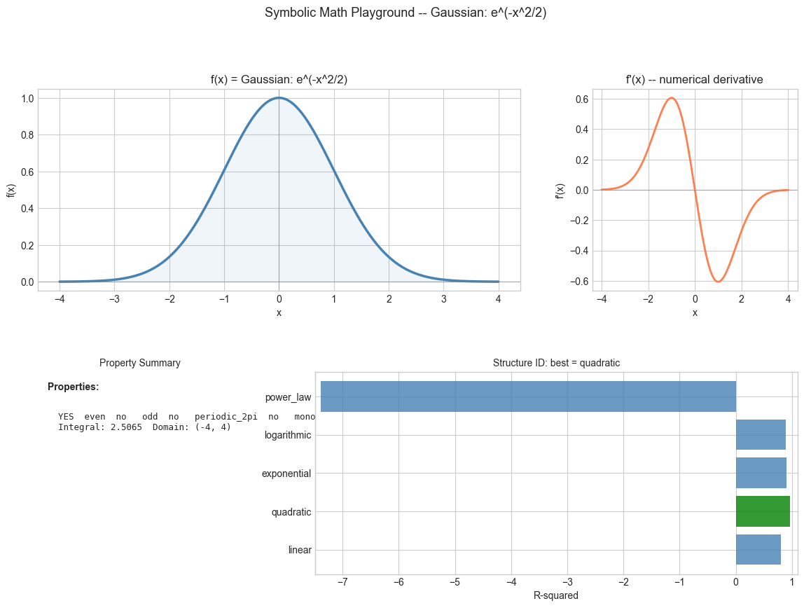
Property report: Gaussian: e^(-x^2/2)
Property                    Holds   Max deviation
--------------------------------------------------
  even                        YES        0.00e+00
  odd                          no        2.00e+00
  periodic_2pi                 no        7.33e-02
  monotone_increasing          no       -6.06e-01
  nonnegative                 YES        3.36e-04
C:\Users\user\AppData\Local\Temp\ipykernel_24988\378153234.py:72: UserWarning: This figure includes Axes that are not compatible with tight_layout, so results might be incorrect.
  plt.tight_layout()
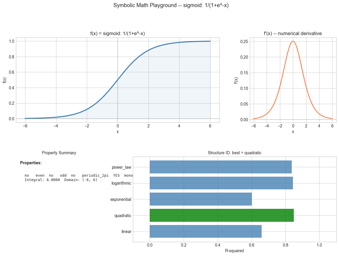
Property report: sigmoid: 1/(1+e^-x)
Property                    Holds   Max deviation
--------------------------------------------------
  even                         no        9.95e-01
  odd                          no        1.00e+00
  periodic_2pi                 no        9.17e-01
  monotone_increasing         YES        2.48e-03
  nonnegative                 YES        2.47e-03
C:\Users\user\AppData\Local\Temp\ipykernel_24988\378153234.py:72: UserWarning: This figure includes Axes that are not compatible with tight_layout, so results might be incorrect.
  plt.tight_layout()
Property report: power: x^1.5
Property                    Holds   Max deviation
--------------------------------------------------
  even                        YES        0.00e+00
  odd                         YES        0.00e+00
  periodic_2pi                 no        2.04e+01
  monotone_increasing         YES        8.13e-02
  nonnegative                 YES        1.43e-05
<string>:1: RuntimeWarning: invalid value encountered in power
C:\Users\user\AppData\Local\Temp\ipykernel_24988\378153234.py:72: UserWarning: This figure includes Axes that are not compatible with tight_layout, so results might be incorrect.
  plt.tight_layout()
7. Results & Reflection
What was built:
A five-component symbolic math playground that:
Represents mathematical expressions as first-class objects with specification and numerical analysis
Tests algebraic properties (even/odd, periodic, monotone, nonnegative) via randomized property testing
Identifies mathematical structure (linear/exponential/power law/logarithmic/quadratic) from data
Generates, tests, and logs mathematical conjectures automatically
Provides a unified visualization dashboard combining all four components
What mathematics made it possible:
Abstraction (ch003): Wrapping expressions in a
MathExpressionclass separates the what (specification) from the how (evaluation)Logical quantifiers (ch012/ch013): Property tests implement for-all quantifiers computationally
Structure identification (ch003/ch008): Log-log regression detects power laws; log-y regression detects exponentials -- each is a linearization of the relevant mathematical structure
Conjecture testing (ch004/ch015/ch016): The engine implements the exploration loop: register claim, test systematically, report outcome
Specification-first programming (ch019): Every class has documented preconditions, postconditions, and properties
Extension challenges:
Add symbolic differentiation. Currently the playground uses numerical derivatives. Extend
MathExpressionto support exact symbolic differentiation for polynomial expressions using the power rule. (Hint: represent polynomials as coefficient arrays and implementsymbolic_derivative(coeffs)that returns the derivative coefficients.)Add the composition operator. Implement
compose(f, g)that creates a newMathExpressionrepresentingf(g(x)). Test it on the chain rule: if h = compose(f, g), then h’(x) should equal f’(g(x)) * g’(x). Verify this numerically for several (f, g) pairs.Extend structure identification to 2D. Currently the identifier only handles univariate data. Extend it to handle bivariate data (x1, x2, y): detect whether y is better described by y = ax1 + bx2 + c (linear plane), y = x1^a * x2^b (power law surface), or y = exp(ax1 + bx2) (exponential surface). Test on synthetic data from each structure.