Prerequisites: ch026 (Real Numbers — IEEE 754 structure), ch036 (Scientific Notation — mantissa/exponent), ch037 (Large Numbers — float64 precision limits) You will learn:
What machine epsilon is and how to measure it
The four sources of floating-point error: rounding, cancellation, overflow, underflow
How to quantify error: absolute error, relative error, ULPs
Techniques to reduce floating-point error: compensated summation, algebraic reformulation
How to recognize when a computation is numerically ill-conditioned
Environment: Python 3.x, numpy, matplotlib
1. Concept
Floating-point arithmetic is not exact. Every operation can introduce a small error. These errors are usually harmless, but they accumulate — and in the wrong computation they compound into results that are completely wrong.
The four sources of floating-point error:
Rounding error. Most real numbers cannot be represented exactly in binary.
0.1in float64 is actually0.1000000000000000055511151231257827021181583404541015625. Every store to a float variable rounds to the nearest representable value.Catastrophic cancellation. Subtracting two nearly equal numbers destroys significant digits.
(1 + ε) - 1returns 0 if ε < machine epsilon.Overflow/Underflow. Numbers too large become
inf; numbers too small become0.0. (covered in ch036, ch037)Accumulation. Summing many small errors in the same direction produces a large total error. Sorting numbers before summing reduces this.
Why this matters for ML: Gradient computations, loss functions, and softmax all involve operations where cancellation and accumulation are active threats. The log-sum-exp trick exists precisely to avoid this.
Common misconceptions:
Float arithmetic is not random — it is deterministic and follows IEEE 754 rules. The errors are small but predictable.
assert a == bfor floats is almost always wrong. Useabs(a - b) < tolerance.Increasing precision (float32 → float64 → float128) reduces error but does not eliminate it. The same structural problems remain.
2. Intuition & Mental Models
Physical analogy: Floating-point numbers are like measuring with a ruler that has marks only at specific positions. The positions are not evenly spaced — they are denser near 0 and sparser near large values. When you measure 1,000,000.1 meters, the ruler’s nearest mark might be at exactly 1,000,000.0 — the 0.1 is lost because there is no mark there at that scale.
Computational analogy: Think of the float64 mantissa as a 53-bit integer. When you add a number with a much smaller exponent, the smaller number’s bits must be right-shifted to align exponents. If the shift exceeds 53, all its bits fall off the end — the number is completely absorbed.
The spacing model: The key insight is that floating-point numbers are not uniformly spaced. In the interval [1, 2), the spacing between adjacent floats is exactly ε_m (machine epsilon ≈ 2.2 × 10⁻¹⁶). In [2, 4), the spacing doubles to 2ε_m. In [0.5, 1), the spacing is ε_m/2. This means: the relative error is approximately constant (~ε_m/2), but the absolute error varies with scale.
Recall from ch036 (Scientific Notation): the mantissa carries 52 explicit bits + 1 implicit leading bit = 53 bits of precision. Machine epsilon = 2⁻⁵² ≈ 2.22 × 10⁻¹⁶ is the gap between 1.0 and the next representable float.
3. Visualization
# --- Visualization: Float spacing is not uniform ---
# Adjacent floats in [1,2) are spaced epsilon_m apart.
# Adjacent floats in [2,4) are spaced 2*epsilon_m apart.
# This shows why relative error is constant but absolute error grows with scale.

import numpy as np
import matplotlib.pyplot as plt

plt.style.use('seaborn-v0_8-whitegrid')

def spacing_at(x):
    """Return the gap between x and the next representable float above x."""
    return np.nextafter(x, np.inf) - x

# Compute spacing across a wide range
base_values = [2**k for k in range(-10, 11)]
spacings = [spacing_at(v) for v in base_values]
relative_spacings = [s / v for s, v in zip(spacings, base_values)]

fig, axes = plt.subplots(1, 2, figsize=(13, 5))

exponents = list(range(-10, 11))
ax1 = axes[0]
ax1.semilogy(exponents, spacings, 'o-', color='crimson', markersize=6)
ax1.set_xlabel('Exponent k  (value = 2^k)', fontsize=11)
ax1.set_ylabel('Absolute spacing (gap to next float)', fontsize=11)
ax1.set_title('Absolute float spacing grows with scale', fontsize=11)

ax2 = axes[1]
ax2.semilogy(exponents, relative_spacings, 'o-', color='steelblue', markersize=6)
ax2.axhline(np.finfo(float).eps, color='darkorange', linestyle='--', linewidth=1.5, label='Machine epsilon (ε_m)')
ax2.set_xlabel('Exponent k  (value = 2^k)', fontsize=11)
ax2.set_ylabel('Relative spacing (gap / value)', fontsize=11)
ax2.set_title('Relative float spacing is constant (~ε_m)', fontsize=11)
ax2.legend(fontsize=10)

plt.suptitle('Float64 spacing: absolute grows, relative stays constant', fontsize=12, fontweight='bold')
plt.tight_layout()
plt.show()

print(f"Machine epsilon: {np.finfo(float).eps:.4e}")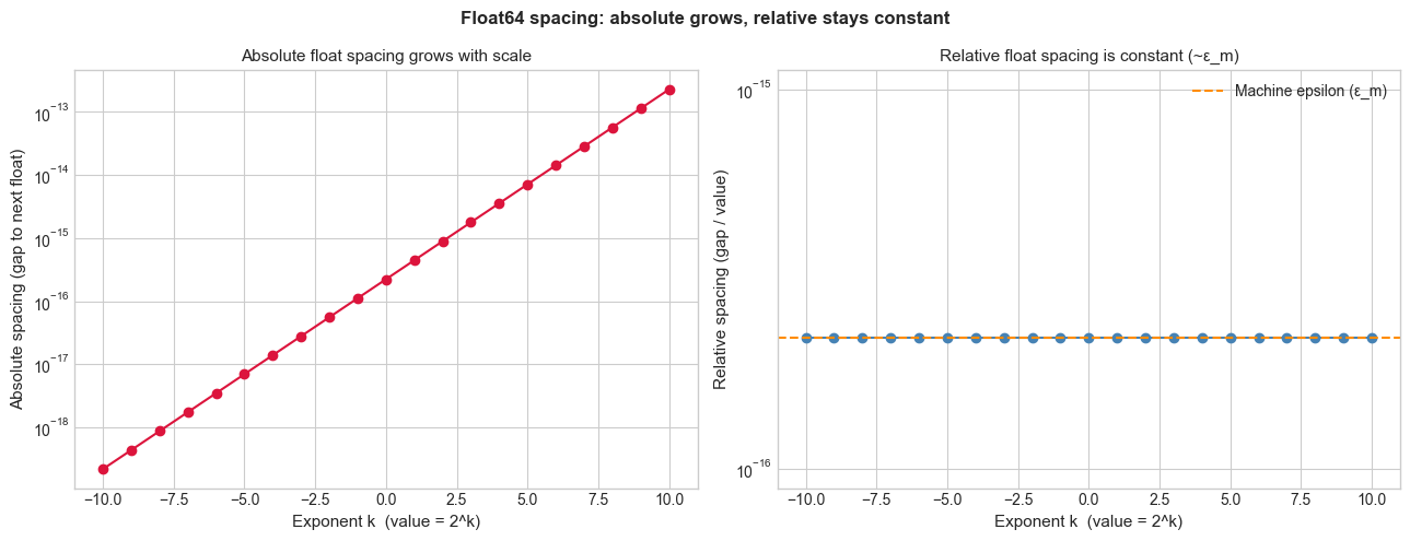
Machine epsilon: 2.2204e-16
# --- Visualization: Catastrophic cancellation ---
# Subtracting nearly-equal numbers destroys significant digits.
# f(x) = (1 - cos(x)) / x^2 should approach 0.5 as x -> 0.
# For small x, direct computation suffers catastrophic cancellation.
# The algebraically equivalent form (sin(x)/x)^2 / (1 + cos(x)) is stable.

import numpy as np
import matplotlib.pyplot as plt

plt.style.use('seaborn-v0_8-whitegrid')

x_values = np.logspace(-16, -1, 400)

# Unstable: direct formula
f_unstable = (1 - np.cos(x_values)) / x_values**2

# Stable: algebraically equivalent using half-angle identity
# (1 - cos x) = 2*sin^2(x/2)  →  f(x) = 2*sin^2(x/2) / x^2
f_stable = 2 * np.sin(x_values / 2)**2 / x_values**2

fig, ax = plt.subplots(figsize=(10, 5))
ax.semilogx(x_values, f_unstable, color='crimson', linewidth=1.5, alpha=0.8, label='Unstable: (1-cos x)/x²')
ax.semilogx(x_values, f_stable, color='steelblue', linewidth=2, label='Stable: 2sin²(x/2)/x²')
ax.axhline(0.5, color='green', linestyle='--', linewidth=1.5, label='True limit = 0.5')
ax.set_xlabel('x', fontsize=11)
ax.set_ylabel('f(x)', fontsize=11)
ax.set_title('Catastrophic cancellation: both formulas are algebraically equal, but only one is numerically stable', fontsize=10)
ax.set_ylim(-0.5, 2.0)
ax.legend(fontsize=10)
plt.tight_layout()
plt.show()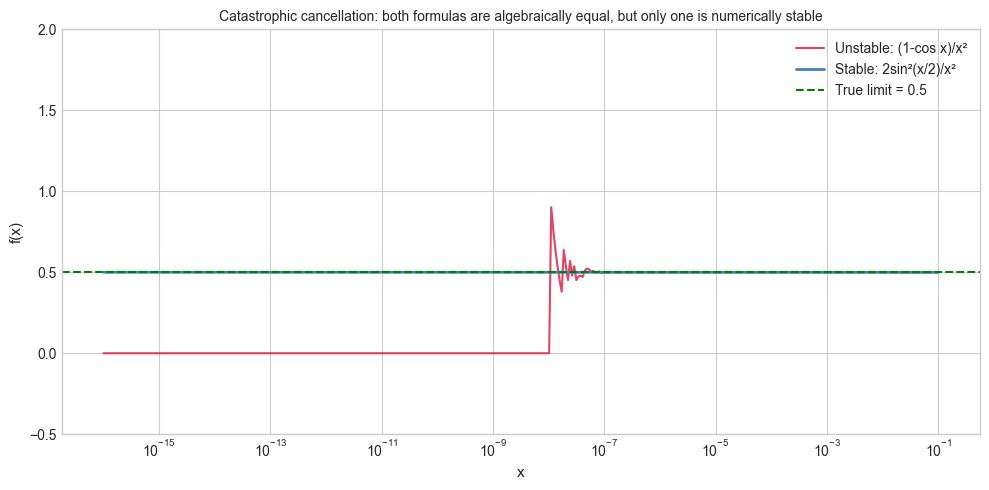
4. Mathematical Formulation
Machine epsilon (ε_m). The smallest float ε such that 1.0 + ε ≠ 1.0:
Every floating-point operation fl(x ⊕ y) satisfies:
The relative error per operation is bounded by ε_m/2.
Absolute and relative error:
Condition number. For a function f, the condition number κ measures how much output error amplifies input error:
A large κ means small input perturbations cause large output changes — the problem is ill-conditioned. Example: f(x) = 1 − cos(x) near x=0 has large κ.
ULP (Unit in the Last Place). The distance between a float and the next representable float. 1 ULP at value x is spacing_at(x). Error measured in ULPs is scale-independent and the IEEE standard guarantees correctly-rounded results within 0.5 ULP for basic operations (+, −, ×, ÷, √).
Compensated (Kahan) summation. Maintains a running compensation term c that captures the rounding error from each step:
This reduces accumulated rounding error from O(nε_m) to O(ε_m) — independent of n.
5. Python Implementation
# --- Implementation: Floating-Point Error Toolkit ---

import numpy as np
import math

def machine_epsilon():
    """
    Compute machine epsilon empirically: smallest e > 0 such that 1.0 + e != 1.0.

    Returns:
        Machine epsilon for float64
    """
    e = 1.0
    while 1.0 + e != 1.0:
        e /= 2.0
    return e * 2  # last e that still caused a difference


def relative_error(computed, true_value):
    """
    Compute relative error between a computed and true value.

    Args:
        computed: numerically computed value
        true_value: exact/reference value (non-zero)

    Returns:
        Relative error = |computed - true| / |true|
    """
    return abs(computed - true_value) / abs(true_value)


def kahan_sum(values):
    """
    Kahan compensated summation — reduces floating-point accumulation error.

    Args:
        values: iterable of floats

    Returns:
        Sum with O(epsilon_m) error regardless of array length
    """
    s = 0.0   # running sum
    c = 0.0   # compensation term (captures lost low-order bits)
    for x in values:
        y = x - c          # apply compensation
        t = s + y          # add (some low-order bits of y are lost here)
        c = (t - s) - y    # recover what was lost: (t-s) should equal y, the difference is the lost bits
        s = t
    return s


def count_ulps(a, b):
    """
    Count the number of ULPs (units in the last place) between two floats.
    Useful for measuring how far two floats are from each other.

    Args:
        a, b: floats of the same sign

    Returns:
        Number of representable floats between a and b
    """
    import struct
    def to_int(x):
        return struct.unpack('Q', struct.pack('d', x))[0]  # interpret bits as uint64
    return abs(to_int(a) - to_int(b))


# --- Validation ---
eps_empirical = machine_epsilon()
eps_numpy = np.finfo(float).eps
print(f"Machine epsilon (empirical):  {eps_empirical:.4e}")
print(f"Machine epsilon (numpy):      {eps_numpy:.4e}")
print(f"Theoretical: 2^-52 =          {2**-52:.4e}")

print()
# Kahan vs naive summation
n = 1_000_000
big = 1.0
small = 1e-8
arr = [big] + [small] * n
naive = sum(arr)
kahan = kahan_sum(arr)
exact = big + small * n  # exact in Python (uses arbitrary precision for the integer part)
print(f"Sum of 1.0 + {n} × 1e-8:")
print(f"  Naive:  {naive:.10f}")
print(f"  Kahan:  {kahan:.10f}")
print(f"  math.fsum: {math.fsum(arr):.10f}")
print(f"  Exact:  {big + n * small:.10f}")

print()
# ULP distance
a = 1.0
b = 1.0 + np.finfo(float).eps
print(f"ULP distance between 1.0 and 1.0+eps: {count_ulps(a, b)}")
print(f"ULP distance between 1.0 and 1.0+2*eps: {count_ulps(a, 1.0 + 2*np.finfo(float).eps)}")
Machine epsilon (empirical): 2.2204e-16
Machine epsilon (numpy): 2.2204e-16
Theoretical: 2^-52 = 2.2204e-16
Sum of 1.0 + 1000000 × 1e-8:
Naive: 1.0100000000
Kahan: 1.0100000000
math.fsum: 1.0100000000
Exact: 1.0100000000
ULP distance between 1.0 and 1.0+eps: 1
ULP distance between 1.0 and 1.0+2*eps: 2
6. Experiments
# --- Experiment 1: Error accumulation vs summation order ---
# Hypothesis: Summing a sorted array (small to large) gives better results
# than summing unsorted because it avoids large+small cancellation.
# Try changing: N and DISTRIBUTION.

import numpy as np
import math

N = 100_000          # <-- modify this
DISTRIBUTION = 'uniform'  # <-- modify this: 'uniform', 'exponential', 'mixed'

rng = np.random.default_rng(42)
if DISTRIBUTION == 'uniform':
    arr = rng.uniform(0, 1, N)
elif DISTRIBUTION == 'exponential':
    arr = rng.exponential(1.0, N)
elif DISTRIBUTION == 'mixed':
    arr = np.concatenate([rng.uniform(1e6, 2e6, N // 2), rng.uniform(0, 1, N // 2)])

exact = math.fsum(arr)  # nearly exact (uses extended precision)

naive_error = abs(np.sum(arr) - exact) / abs(exact)
sorted_error = abs(np.sum(np.sort(arr)) - exact) / abs(exact)
kahan_error = abs(kahan_sum(arr) - exact) / abs(exact)

print(f"N = {N}, distribution = {DISTRIBUTION}")
print(f"Exact (fsum):   {exact:.10f}")
print(f"Naive sum:      relative error = {naive_error:.2e}")
print(f"Sorted sum:     relative error = {sorted_error:.2e}")
print(f"Kahan sum:      relative error = {kahan_error:.2e}")
N = 100000, distribution = uniform
Exact (fsum): 50062.4936662159
Naive sum: relative error = 0.00e+00
Sorted sum: relative error = 1.45e-16
Kahan sum: relative error = 0.00e+00
# --- Experiment 2: The classic 0.1 + 0.2 != 0.3 ---
# Hypothesis: 0.1, 0.2, 0.3 cannot be represented exactly in binary.
# The 'error' is at the 17th decimal digit, below practical significance.
# But it breaks equality checks — a lesson in floating-point comparison.

a = 0.1
b = 0.2
c = 0.3
result = a + b

print("=== 0.1 + 0.2 == 0.3? ===")
print(f"0.1 = {a:.20f}")
print(f"0.2 = {b:.20f}")
print(f"0.3 = {c:.20f}")
print(f"0.1 + 0.2 = {result:.20f}")
print(f"0.1 + 0.2 == 0.3: {result == c}")
print(f"Difference: {result - c:.4e}")
print()

TOLERANCE = 1e-9  # <-- modify this
print(f"abs(result - 0.3) < {TOLERANCE}: {abs(result - c) < TOLERANCE}")
print(f"np.isclose(result, 0.3):          {np.isclose(result, c)}")
print()
print("np.isclose uses rtol=1e-5, atol=1e-8 by default — a sensible practical threshold.")
=== 0.1 + 0.2 == 0.3? ===
0.1 = 0.10000000000000000555
0.2 = 0.20000000000000001110
0.3 = 0.29999999999999998890
0.1 + 0.2 = 0.30000000000000004441
0.1 + 0.2 == 0.3: False
Difference: 5.5511e-17
abs(result - 0.3) < 1e-09: True
np.isclose(result, 0.3): True
np.isclose uses rtol=1e-5, atol=1e-8 by default — a sensible practical threshold.
# --- Experiment 3: Quadratic formula — unstable vs stable ---
# Hypothesis: for b >> sqrt(b^2 - 4ac), the standard formula suffers
# catastrophic cancellation. The numerically stable form avoids it.
# Try changing: a, b, c to near-degenerate cases.

import numpy as np

# Coefficients: ax^2 + bx + c = 0
a = 1.0
b = -1e8    # <-- modify this (large b causes cancellation)
c = 1.0

# Standard formula: x = (-b ± sqrt(b^2 - 4ac)) / 2a
discriminant = b**2 - 4*a*c
x1_std = (-b + np.sqrt(discriminant)) / (2*a)
x2_std = (-b - np.sqrt(discriminant)) / (2*a)

# Stable formula: avoid cancellation by using the larger root first,
# then apply Vieta's formula (x1 * x2 = c/a) to get the other.
if b >= 0:
    x1_stable = (-b - np.sqrt(discriminant)) / (2*a)
else:
    x1_stable = (-b + np.sqrt(discriminant)) / (2*a)
x2_stable = c / (a * x1_stable)   # Vieta: x1 * x2 = c/a

# Verify with Python's high-precision: exact roots via quadratic formula in python int
# For large b, one root ≈ b/a, other ≈ c/(b/a) = ac/b
x1_exact_approx = -b / a  # dominant root
x2_exact_approx = c / (b * (-1))  # small root via Vieta

print(f"Coefficients: a={a}, b={b}, c={c}")
print(f"\nStandard formula:")
print(f"  x1 = {x1_std:.10f}")
print(f"  x2 = {x2_std:.10e}   ← potential cancellation error")
print(f"\nStable formula:")
print(f"  x1 = {x1_stable:.10f}")
print(f"  x2 = {x2_stable:.10e}   ← stable via Vieta's formulas")
print(f"\nApprox exact:")
print(f"  x2 ≈ {x2_exact_approx:.10e}")
print(f"\nRelative error in x2:")
print(f"  Standard: {abs(x2_std - x2_exact_approx)/abs(x2_exact_approx):.4e}")
print(f"  Stable:   {abs(x2_stable - x2_exact_approx)/abs(x2_exact_approx):.4e}")
Coefficients: a=1.0, b=-100000000.0, c=1.0
Standard formula:
x1 = 100000000.0000000000
x2 = 7.4505805969e-09 ← potential cancellation error
Stable formula:
x1 = 100000000.0000000000
x2 = 1.0000000000e-08 ← stable via Vieta's formulas
Approx exact:
x2 ≈ 1.0000000000e-08
Relative error in x2:
Standard: 2.5494e-01
Stable: 0.0000e+00
7. Exercises
Easy 1. Compute machine epsilon empirically for float32 (use np.float32 arithmetic). Compare it to the theoretical value 2⁻²³. How many fewer significant decimal digits does float32 offer compared to float64? (Expected: a single float and integer)
Easy 2. Write a function is_close(a, b, rel_tol=1e-9, abs_tol=0.0) that returns True if |a - b| <= max(rel_tol * max(|a|, |b|), abs_tol). Test it on: is_close(0.1 + 0.2, 0.3) and is_close(1e-15, 2e-15). (This is essentially what math.isclose implements)
Medium 1. The harmonic series H_n = 1 + 1/2 + 1/3 + ... + 1/n. Compute H_10000000 (ten million terms) using: (a) naive sum from 1 to n, (b) summing from n down to 1 (small to large), (c) Kahan summation. Compare results and explain which is most accurate and why.
Medium 2. Investigate the log-sum-exp trick, used in ML for numerically stable softmax. Implement log_sum_exp(x_array) both naively (log(sum(exp(x)))) and stably (subtract max first). Test for arrays with large values like [1000, 1001, 1002] — the naive version overflows to inf; the stable version should not.
Hard. Implement a simple interval arithmetic library: represent each number as an interval [lo, hi] that is guaranteed to contain the true value. Implement +, −, ×, ÷ for intervals (use np.nextafter to round outward). Test it on ((1/3 + 1/7) * 21) — the exact answer is 10, and your interval should contain 10.0. This is the basis of verified numerical computing.
8. Mini Project — Numerical Stability Audit
# --- Mini Project: Numerical Stability Audit of Common Formulas ---
# Problem:
#   Many formulas that are mathematically correct are numerically unstable.
#   Build a tool that computes several standard formulas in both their
#   naive and numerically stable forms, and plots the relative error
#   as a function of input magnitude.
#
# Formulas to audit:
#   1. (1 - cos x) / x^2  vs  2*sin^2(x/2) / x^2   (limit = 0.5)
#   2. sqrt(x+1) - sqrt(x)  vs  1 / (sqrt(x+1) + sqrt(x))  (equivalent by rationalization)
#   3. exp(x) - 1  vs  np.expm1(x)  (for small x)

import numpy as np
import matplotlib.pyplot as plt

plt.style.use('seaborn-v0_8-whitegrid')

# --- Formula 1: (1 - cos x) / x^2 ---
x_small = np.logspace(-16, -1, 500)
f1_naive = (1 - np.cos(x_small)) / x_small**2
f1_stable = 2 * np.sin(x_small/2)**2 / x_small**2  # half-angle identity
f1_true = 0.5  # limit as x->0

# --- Formula 2: sqrt(x+1) - sqrt(x) ---
x_large = np.logspace(0, 14, 500)
f2_naive = np.sqrt(x_large + 1) - np.sqrt(x_large)
f2_stable = 1.0 / (np.sqrt(x_large + 1) + np.sqrt(x_large))  # rationalized
f2_true = f2_stable  # stable form is essentially exact here

# --- Formula 3: e^x - 1 for small x ---
x_tiny = np.logspace(-16, -1, 500)
f3_naive = np.exp(x_tiny) - 1
f3_stable = np.expm1(x_tiny)   # built-in stable implementation
f3_true = x_tiny + x_tiny**2/2 + x_tiny**3/6  # Taylor approx (essentially exact for small x)

fig, axes = plt.subplots(1, 3, figsize=(16, 5))

# Plot relative errors
err1_naive = np.abs(f1_naive - f1_true) / abs(f1_true)
err1_stable = np.abs(f1_stable - f1_true) / abs(f1_true)
axes[0].loglog(x_small, err1_naive + 1e-18, color='crimson', lw=1.5, label='Naive')
axes[0].loglog(x_small, err1_stable + 1e-18, color='steelblue', lw=1.5, label='Stable')
axes[0].set_title('(1-cos x)/x²  (limit=0.5)', fontsize=10)
axes[0].set_xlabel('x'); axes[0].set_ylabel('Relative error'); axes[0].legend()

err2_naive = np.abs(f2_naive - f2_true) / (np.abs(f2_true) + 1e-300)
axes[1].loglog(x_large, err2_naive + 1e-18, color='crimson', lw=1.5, label='Naive')
axes[1].axhline(np.finfo(float).eps, color='steelblue', linestyle='--', lw=1.5, label='ε_m (stable floor)')
axes[1].set_title('√(x+1) - √x  vs  rationalized', fontsize=10)
axes[1].set_xlabel('x'); axes[1].set_ylabel('Relative error'); axes[1].legend()

err3_naive = np.abs(f3_naive - f3_true) / (np.abs(f3_true) + 1e-300)
err3_stable = np.abs(f3_stable - f3_true) / (np.abs(f3_true) + 1e-300)
axes[2].loglog(x_tiny, err3_naive + 1e-18, color='crimson', lw=1.5, label='exp(x)-1 (naive)')
axes[2].loglog(x_tiny, err3_stable + 1e-18, color='steelblue', lw=1.5, label='expm1(x) (stable)')
axes[2].set_title('eˣ - 1 for small x', fontsize=10)
axes[2].set_xlabel('x'); axes[2].set_ylabel('Relative error'); axes[2].legend()

plt.suptitle('Numerical stability audit: naive vs stable formulas', fontsize=12, fontweight='bold')
plt.tight_layout()
plt.show()

# TODO: Add a fourth formula of your choice and audit it.
9. Chapter Summary & Connections
What was covered:
Machine epsilon ε_m ≈ 2.22 × 10⁻¹⁶ is the fundamental precision unit for float64: the relative spacing between adjacent representable values is constant at ε_m.
Rounding, cancellation, accumulation, and overflow/underflow are the four sources of floating-point error.
Catastrophic cancellation occurs when subtracting nearly equal values; algebraic reformulation (half-angle, Vieta’s, rationalization) eliminates it.
Kahan summation reduces accumulated error from O(nε_m) to O(ε_m) at constant overhead.
Condition number κ measures intrinsic problem sensitivity — distinguishing numerical instability (implementation flaw) from ill-conditioning (mathematical fact).
Backward connection: This chapter formalizes the precision limits introduced informally in ch026 (Real Numbers) and ch036 (Scientific Notation), and connects to the catastrophic cancellation preview in ch037 (Large Numbers).
Forward connections:
(ch039 — Numerical Stability): extends precision analysis to iterative algorithms — when do errors grow vs decay over iterations? Covers stable recurrences, Gram-Schmidt orthogonalization, and forward vs backward stability.
(ch207 — Numerical Derivatives): finite difference approximations for derivatives are directly limited by machine epsilon — the optimal step size is O(√ε_m), a direct consequence of this chapter.
(ch212 — Gradient Descent): the log-sum-exp trick and numerically stable softmax are floating-point techniques that come directly from the cancellation analysis here.
Going deeper: Accuracy and Stability of Numerical Algorithms by Nicholas Higham (2nd ed.) is the definitive reference. For the IEEE 754 standard itself, the original Goldberg paper (What Every Computer Scientist Should Know About Floating-Point Arithmetic, 1991) remains freely available.