Prerequisites: ch022 (Natural Numbers), ch023 (Integers), ch026 (Real Numbers), ch031 (Modular Arithmetic)
You will learn:
What exponentiation is and why it differs fundamentally from multiplication
Integer, rational, and real exponents — and what each generalizes
How computers compute powers efficiently (fast exponentiation)
The mathematical rules (laws of exponents) and where they break down
Connections to growth, scientific notation, and algorithm complexity
Environment: Python 3.x, numpy, matplotlib
1. Concept
Exponentiation answers the question: what happens when you apply multiplication the way multiplication applies addition?
Addition: combine equal groups of 1 →
n + n + n = 3n(multiplication)Multiplication: combine equal groups of n →
n × n × n = n³(exponentiation)
The expression b^n (read: b to the power n) means: multiply b by itself n times.
2^1 = 2
2^2 = 2 × 2 = 4
2^3 = 2 × 2 × 2 = 8
2^10 = 1024
2^32 = 4,294,967,296
The growth rate here is qualitatively different from addition or multiplication. Each increment of the exponent multiplies the result, not adds to it.
Terminology:
bis the basenis the exponent (or power)The result is a power of b
Common misconception: b^n is not b × n. Students write 2^3 = 6 (confusing with 2 × 3). The exponent tells you how many times to use b as a factor, not how many times to add it.
Scope of this chapter: We focus on the structure and laws of exponentiation — integer, then rational, then real exponents. The behavior of exponential functions (growth, decay, rates) is covered in ch042.
2. Intuition & Mental Models
Geometric analogy: Think of b^n as measuring n-dimensional volume with side length b.
b^1= a line segment of length bb^2= a square with side b (area)b^3= a cube with side b (volume)b^4and beyond = a hypercube (you can’t picture it, but the math still works)
This is why b^2 is called “b squared” and b^3 is “b cubed” — literal geometric origins.
Computational analogy: Think of b^n as a chain of multiplications. A computer implementing pow(b, n) naively does exactly n-1 multiplications. But — and this is important — there’s a smarter way. We’ll implement it in Section 5.
Fractional exponents: b^(1/2) = the number that, when squared, gives b. That’s the square root. So b^(1/n) = the n-th root of b. Exponentiation and root-taking are inverses (this will become precise in ch043 — Logarithms Intuition).
Negative exponents: b^(-n) = 1 / b^n. Think of it as “going in reverse” on the multiplication chain. 2^3 = 8, so 2^(-3) = 1/8. (Introduced in the context of rational numbers in ch024.)
Zero exponent: b^0 = 1 for any b ≠ 0. This follows from the division rule: b^n / b^n = b^(n-n) = b^0, and any number divided by itself is 1.
3. Visualization
# --- Visualization: Exponent landscape — how b^n behaves across bases and exponents ---
import numpy as np
import matplotlib.pyplot as plt

plt.style.use('seaborn-v0_8-whitegrid')

fig, axes = plt.subplots(1, 3, figsize=(15, 5))

# --- Panel 1: b^n for fixed base b, varying exponent n ---
ax = axes[0]
exponents = np.arange(0, 11)
for base in [2, 3, 10]:
    values = base ** exponents
    ax.plot(exponents, values, marker='o', label=f'base = {base}')
ax.set_title('b^n: Fixed Base, Varying Exponent')
ax.set_xlabel('Exponent n')
ax.set_ylabel('b^n')
ax.legend()

# --- Panel 2: b^n for fixed exponent n, varying base b ---
ax = axes[1]
bases = np.linspace(0.1, 4, 200)
for exp in [1, 2, 3, 4]:
    ax.plot(bases, bases ** exp, label=f'n = {exp}')
ax.set_title('b^n: Fixed Exponent, Varying Base')
ax.set_xlabel('Base b')
ax.set_ylabel('b^n')
ax.legend()
ax.set_ylim(0, 20)

# --- Panel 3: Negative and fractional exponents ---
ax = axes[2]
exps = np.linspace(-3, 3, 300)
for base in [2, 0.5]:
    ax.plot(exps, base ** exps, label=f'base = {base}')
ax.axhline(1, color='gray', linestyle='--', linewidth=0.8, label='y = 1 (any b^0)')
ax.set_title('b^n: Fractional and Negative Exponents')
ax.set_xlabel('Exponent n (real-valued)')
ax.set_ylabel('b^n')
ax.legend()

plt.suptitle('Exponentiation: Landscape Across Bases and Exponents', fontsize=14, y=1.02)
plt.tight_layout()
plt.show()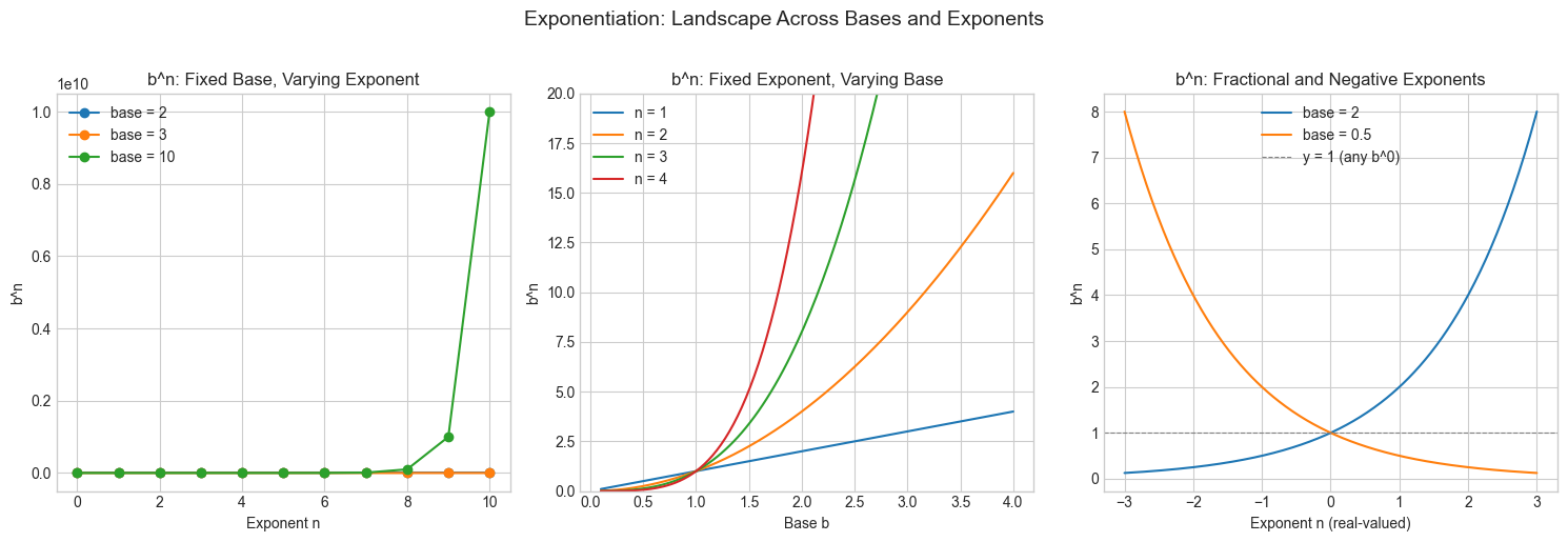
# --- Visualization: The geometric interpretation (squares and cubes) ---
import matplotlib.patches as patches

fig, axes = plt.subplots(1, 3, figsize=(12, 4))

BASE = 3  # b = 3

# b^1: line
ax = axes[0]
ax.plot([0, BASE], [0.5, 0.5], 'b-', linewidth=6)
ax.set_xlim(-0.5, BASE + 0.5)
ax.set_ylim(0, 1)
ax.set_title(f'b^1 = {BASE}^1 = {BASE}\n(length)')
ax.set_xlabel('units')
ax.set_yticks([])

# b^2: square
ax = axes[1]
square = patches.Rectangle((0, 0), BASE, BASE, linewidth=1.5,
                             edgecolor='blue', facecolor='lightblue', alpha=0.5)
ax.add_patch(square)
ax.set_xlim(-0.5, BASE + 0.5)
ax.set_ylim(-0.5, BASE + 0.5)
ax.set_aspect('equal')
ax.set_title(f'b^2 = {BASE}^2 = {BASE**2}\n(area)')
ax.set_xlabel('units')
ax.set_ylabel('units')

# b^n: value plot showing geometric growth
ax = axes[2]
ns = np.arange(0, 7)
vals = BASE ** ns
ax.bar(ns, vals, color='steelblue', alpha=0.7)
for i, v in zip(ns, vals):
    ax.text(i, v + 0.5, str(v), ha='center', fontsize=9)
ax.set_title(f'b^n for b={BASE}, n=0..6')
ax.set_xlabel('Exponent n')
ax.set_ylabel('Value')

plt.tight_layout()
plt.show()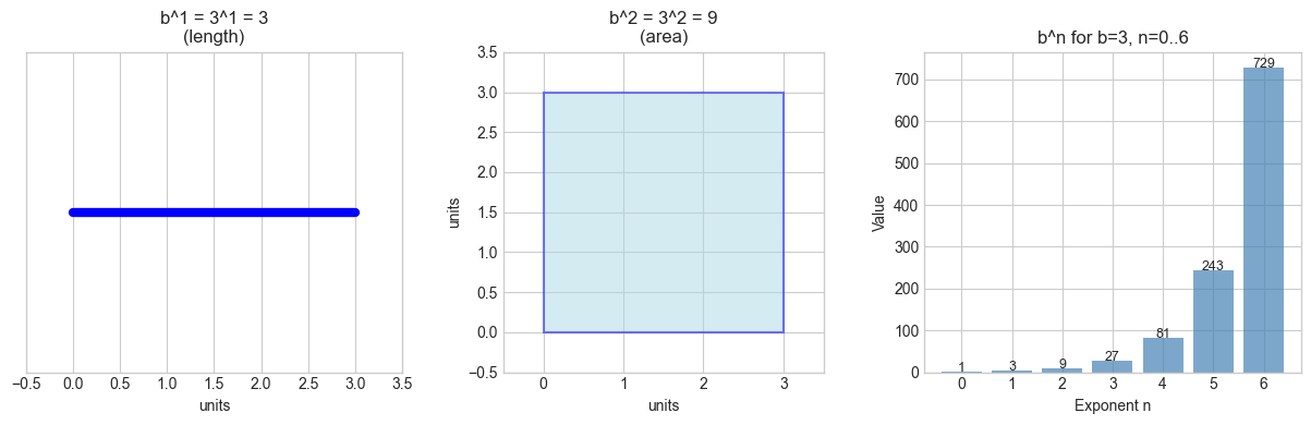
4. Mathematical Formulation
Definition for integer exponents
For b ∈ ℝ, n ∈ ℕ (positive integer):
b^n = b × b × b × ... × b    (n times)
b^0 = 1                        (by convention, b ≠ 0)
b^(-n) = 1 / b^n               (n > 0, b ≠ 0)
Laws of exponents
These follow directly from the definition. Let b, c > 0 and m, n ∈ ℝ:
1.  b^m × b^n = b^(m+n)        # product rule: count the factors
2.  b^m / b^n = b^(m-n)        # quotient rule: cancel common factors
3.  (b^m)^n  = b^(m×n)         # power of a power: flatten the nesting
4.  (b×c)^n  = b^n × c^n       # distribute over multiplication
5.  (b/c)^n  = b^n / c^n       # distribute over division
Extension to rational exponents
For p/q in lowest terms, q > 0, b > 0:
b^(p/q) = (b^(1/q))^p = (q-th root of b)^pExample: 8^(2/3) = (cube_root(8))^2 = 2^2 = 4
Extension to real exponents
For irrational exponents (like 2^π), the definition requires limits (covered in ch201 — Limits Intuition):
b^x = lim_{r→x, r rational} b^rIn practice: compute via exp(x × ln(b)) — the natural logarithm and exponential function (ch043, ch044).
# --- Verify laws of exponents numerically ---
import numpy as np

b, c = 3.0, 2.0
m, n = 4.0, 3.0

print("Laws of Exponents — Numerical Verification")
print("-" * 50)

# Law 1: b^m × b^n = b^(m+n)
lhs = b**m * b**n
rhs = b**(m + n)
print(f"1. b^m × b^n = b^(m+n):  {lhs:.4f} == {rhs:.4f}  {'✓' if np.isclose(lhs, rhs) else '✗'}")

# Law 2: b^m / b^n = b^(m-n)
lhs = b**m / b**n
rhs = b**(m - n)
print(f"2. b^m / b^n = b^(m-n):  {lhs:.4f} == {rhs:.4f}  {'✓' if np.isclose(lhs, rhs) else '✗'}")

# Law 3: (b^m)^n = b^(m×n)
lhs = (b**m)**n
rhs = b**(m * n)
print(f"3. (b^m)^n  = b^(m×n):   {lhs:.4f} == {rhs:.4f}  {'✓' if np.isclose(lhs, rhs) else '✗'}")

# Law 4: (b×c)^n = b^n × c^n
lhs = (b * c)**n
rhs = b**n * c**n
print(f"4. (b×c)^n = b^n × c^n: {lhs:.4f} == {rhs:.4f}  {'✓' if np.isclose(lhs, rhs) else '✗'}")

# Rational exponent: 8^(2/3)
val = 8 ** (2/3)
expected = 4.0
print(f"\nRational: 8^(2/3) = {val:.6f}  (expected {expected})  {'✓' if np.isclose(val, expected) else '✗'}")

# Real exponent: 2^π via exp(π × ln(2))
val_direct = 2 ** np.pi
val_via_exp = np.exp(np.pi * np.log(2))
print(f"Real: 2^π = {val_direct:.8f}  via exp(π×ln2) = {val_via_exp:.8f}  {'✓' if np.isclose(val_direct, val_via_exp) else '✗'}")
Laws of Exponents — Numerical Verification
--------------------------------------------------
1. b^m × b^n = b^(m+n): 2187.0000 == 2187.0000 ✓
2. b^m / b^n = b^(m-n): 3.0000 == 3.0000 ✓
3. (b^m)^n = b^(m×n): 531441.0000 == 531441.0000 ✓
4. (b×c)^n = b^n × c^n: 216.0000 == 216.0000 ✓
Rational: 8^(2/3) = 4.000000 (expected 4.0) ✓
Real: 2^π = 8.82497783 via exp(π×ln2) = 8.82497783 ✓
5. Python Implementation
Naive vs fast exponentiation
Python’s ** operator and pow() built-in use fast exponentiation internally. Let’s implement both to understand the difference.
# --- Implementation: Naive integer exponentiation ---

def power_naive(base, exp):
    """
    Compute base^exp using repeated multiplication.
    Requires exactly (exp - 1) multiplications.

    Args:
        base: numeric base
        exp: non-negative integer exponent

    Returns:
        base raised to exp
    """
    if exp == 0:
        return 1
    result = 1
    for _ in range(exp):
        result *= base  # multiply exp times
    return result


# --- Implementation: Fast exponentiation (exponentiation by squaring) ---

def power_fast(base, exp):
    """
    Compute base^exp using exponentiation by squaring.
    Requires O(log exp) multiplications instead of O(exp).

    Key insight:
        if exp is even:  base^exp = (base^2)^(exp/2)
        if exp is odd:   base^exp = base × base^(exp-1)

    Args:
        base: numeric base
        exp: non-negative integer exponent

    Returns:
        base raised to exp
    """
    if exp == 0:
        return 1
    if exp % 2 == 0:
        # Even: square the base, halve the exponent
        return power_fast(base * base, exp // 2)
    else:
        # Odd: pull out one factor, recurse on even
        return base * power_fast(base, exp - 1)


# Validate both implementations
test_cases = [(2, 10), (3, 7), (5, 0), (7, 1), (2, 32)]
print("base  exp  naive        fast         python")
print("-" * 55)
for b, e in test_cases:
    naive = power_naive(b, e)
    fast  = power_fast(b, e)
    ref   = b ** e
    match = '✓' if naive == fast == ref else '✗'
    print(f"{b:4d}  {e:3d}  {naive:12d}  {fast:12d}  {ref:12d}  {match}")
base exp naive fast python
-------------------------------------------------------
2 10 1024 1024 1024 ✓
3 7 2187 2187 2187 ✓
5 0 1 1 1 ✓
7 1 7 7 7 ✓
2 32 4294967296 4294967296 4294967296 ✓
# --- Count multiplications: naive vs fast ---

def power_fast_counting(base, exp, count=None):
    """Same as power_fast but counts the number of multiplications."""
    if count is None:
        count = [0]
    if exp == 0:
        return 1, count[0]
    if exp % 2 == 0:
        count[0] += 1  # the squaring: base * base
        result, _ = power_fast_counting(base * base, exp // 2, count)
        return result, count[0]
    else:
        count[0] += 1  # the outer base * ...
        result, _ = power_fast_counting(base, exp - 1, count)
        return result, count[0]

import numpy as np
import matplotlib.pyplot as plt

plt.style.use('seaborn-v0_8-whitegrid')

exponents = np.arange(1, 65)
naive_mults = exponents - 1  # always exp-1 multiplications
fast_mults  = [power_fast_counting(2, int(e))[1] for e in exponents]
log2_bound  = np.log2(exponents) * 2  # theoretical O(log n) bound

fig, ax = plt.subplots(figsize=(9, 5))
ax.plot(exponents, naive_mults, label='Naive: O(n) multiplications', color='tomato')
ax.plot(exponents, fast_mults,  label='Fast: actual multiplications', color='steelblue', marker='.')
ax.plot(exponents, log2_bound,  label='2·log₂(n) bound', color='green', linestyle='--')
ax.set_title('Naive vs Fast Exponentiation: Multiplication Count')
ax.set_xlabel('Exponent n')
ax.set_ylabel('Number of multiplications')
ax.legend()
plt.tight_layout()
plt.show()

print(f"\nFor n=64: naive needs {64-1} multiplications, fast needs {power_fast_counting(2, 64)[1]}")
C:\Users\user\AppData\Local\Temp\ipykernel_23940\1714877022.py:36: UserWarning: Glyph 8322 (\N{SUBSCRIPT TWO}) missing from font(s) Arial.
plt.tight_layout()
c:\Users\user\OneDrive\Documents\book\.venv\Lib\site-packages\IPython\core\pylabtools.py:170: UserWarning: Glyph 8322 (\N{SUBSCRIPT TWO}) missing from font(s) Arial.
fig.canvas.print_figure(bytes_io, **kw)
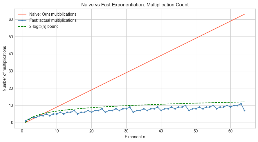
For n=64: naive needs 63 multiplications, fast needs 7
The algorithm’s correctness relies on Law 3 from Section 4: (b^2)^(n/2) = b^(2 × n/2) = b^n.
This same idea powers modular exponentiation, the core of RSA cryptography (introduced in ch031 — Modular Arithmetic, applied in ch033 — Applications of Modulo).
6. Experiments
# --- Experiment 1: Where do the laws of exponents break down? ---
# Hypothesis: The laws assume b > 0 and real exponents.
# Negative bases with fractional exponents cause problems.
# Try changing: BASE to a negative number, EXP to a fraction

import numpy as np

BASE = -8   # <-- modify this (try -2, -1, 0)
EXP  = 1/3  # <-- modify this (try 2, -1, 0.5)

# Python's float arithmetic
try:
    result_float = BASE ** EXP
    print(f"Python float: ({BASE})^({EXP}) = {result_float}")
except Exception as e:
    print(f"Python float error: {e}")

# NumPy's complex-aware version
result_complex = complex(BASE) ** EXP
print(f"Complex result: ({BASE})^({EXP}) = {result_complex}")

# The real cube root of -8 should be -2 (since (-2)^3 = -8)
# Python cannot compute it as a float because x^(1/3) via exp(ln(x)/3)
# requires ln of a negative number — which is complex.
print(f"\nVerification: (-2)^3 = {(-2)**3}")
print(f"So the real cube root of -8 is -2, but Python gives: {BASE**EXP}")
print("This is why the laws require b > 0 for real-valued exponentiation.")
Python float: (-8)^(0.3333333333333333) = (1.0000000000000002+1.7320508075688772j)
Complex result: (-8)^(0.3333333333333333) = (1.0000000000000002+1.7320508075688772j)
Verification: (-2)^3 = -8
So the real cube root of -8 is -2, but Python gives: (1.0000000000000002+1.7320508075688772j)
This is why the laws require b > 0 for real-valued exponentiation.
# --- Experiment 2: Power towers (iterated exponentiation) ---
# Hypothesis: a^(b^c) ≠ (a^b)^c in general — exponentiation is NOT associative.
# Try changing: A, B, C to explore when they happen to be equal

A = 2  # <-- modify this
B = 3  # <-- modify this
C = 2  # <-- modify this

# Right-associative: a^(b^c) — how power towers work by convention
right = A ** (B ** C)

# Left-associative: (a^b)^c — equivalent to a^(b×c) by Law 3
left = (A ** B) ** C

print(f"a={A}, b={B}, c={C}")
print(f"Right-associative: a^(b^c) = {A}^({B}^{C}) = {A}^{B**C} = {right}")
print(f"Left-associative: (a^b)^c  = ({A}^{B})^{C} = {A**B}^{C}  = {left}")
print(f"Equal? {right == left}")
print(f"\nNote: Law 3 says (a^b)^c = a^(b×c) = {A}^{B*C} = {A**(B*C)}")
print(f"But a^(b^c) = a^{B**C} = {right}  — very different for large exponents!")
a=2, b=3, c=2
Right-associative: a^(b^c) = 2^(3^2) = 2^9 = 512
Left-associative: (a^b)^c = (2^3)^2 = 8^2 = 64
Equal? False
Note: Law 3 says (a^b)^c = a^(b×c) = 2^6 = 64
But a^(b^c) = a^9 = 512 — very different for large exponents!
# --- Experiment 3: Modular exponentiation (RSA preview) ---
# Hypothesis: (base^exp) mod m can be computed efficiently WITHOUT
# computing the full (astronomically large) base^exp first.
# This is the core operation in RSA encryption.

BASE = 7
EXP  = 1000    # <-- modify this (try 10_000, 100_000)
MOD  = 13      # <-- modify this (try other primes: 17, 29, 97)

# Python's built-in 3-argument pow is optimized for this
result = pow(BASE, EXP, MOD)  # computes (BASE^EXP) mod MOD efficiently

# Naive: compute the full number first (catastrophically slow for large EXP)
# result_naive = (BASE ** EXP) % MOD  # <-- try this for EXP=1000, then comment out

print(f"({BASE}^{EXP}) mod {MOD} = {result}")
print(f"Using Python's 3-arg pow: O(log {EXP}) ≈ {int(EXP.bit_length())} multiplications")
print(f"The full number {BASE}^{EXP} has ~{int(EXP * len(str(BASE)))} digits — never computed.")
(7^1000) mod 13 = 9
Using Python's 3-arg pow: O(log 1000) ≈ 10 multiplications
The full number 7^1000 has ~1000 digits — never computed.
7. Exercises
Easy 1. Compute 5^6 by hand using the product rule. Verify in Python. Then explain why (5^3)^2 = 5^6 using Law 3.
Easy 2. What is 0^0? In Python, 0**0 returns 1. Is this mathematically correct? Write 2–3 sentences explaining the two competing perspectives (combinatorics vs analysis).
Medium 1. Implement power_fast iteratively (without recursion) using a loop. Verify it produces identical results to the recursive version for all exponents 0–100. (Hint: use the binary representation of the exponent.)
Medium 2. The function f(n) = 2^n grows faster than g(n) = n^2 for large n. Find the crossover point: the smallest integer n where 2^n > n^2. Then find where 2^n > n^10.
Hard. Prove algebraically that the fast exponentiation algorithm is correct. That is, show that power_fast(b, n) returns b^n for all n ≥ 0 by strong induction. State the base case, the inductive hypothesis, and the two cases (even/odd) explicitly.
8. Mini Project: Integer Factorization and Smooth Numbers
# --- Mini Project: Smooth Numbers and the Cost of Representing Powers ---
#
# Problem:
#   A number is called "B-smooth" if all its prime factors are ≤ B.
#   Powers of small primes are the smoothest numbers — and they appear
#   constantly in algorithm analysis (2^n in binary search, 2^32 in
#   32-bit integers, etc.).
#
#   Your task: Build a tool that, given a number N, finds its representation
#   as a product of prime powers, and computes how many bits it needs.
#
# Dataset: Generated inline (integer powers of small primes)
# Task: Factor a number into prime powers, count its bit length, and
#       visualize the relationship between prime-power structure and bit length.

import numpy as np
import matplotlib.pyplot as plt

plt.style.use('seaborn-v0_8-whitegrid')

# --- Starter code: complete the TODOs ---

def prime_factorization(n):
    """
    Return the prime factorization of n as a dict {prime: exponent}.
    Example: prime_factorization(360) → {2: 3, 3: 2, 5: 1}
    """
    factors = {}
    d = 2
    while d * d <= n:
        while n % d == 0:
            factors[d] = factors.get(d, 0) + 1
            n //= d
        d += 1
    if n > 1:
        factors[n] = factors.get(n, 0) + 1
    return factors

def bit_length(n):
    """Number of bits needed to represent n in binary."""
    return n.bit_length()

# TODO 1: Generate 50 numbers that are powers of 2 and 3
#         (i.e., numbers of the form 2^a * 3^b for a,b in 0..10)
#         Hint: nested loop, collect unique values, sort
numbers = sorted(set(
    2**a * 3**b
    for a in range(12)
    for b in range(8)
))

# TODO 2: For each number, compute its bit length and factorization
bit_lengths = [bit_length(n) for n in numbers]
factorizations = [prime_factorization(n) for n in numbers]

# TODO 3: Plot bit_length vs log2(number)
# What do you expect this relationship to look like?
log2_values = np.log2(numbers)

fig, axes = plt.subplots(1, 2, figsize=(13, 5))

ax = axes[0]
ax.scatter(log2_values, bit_lengths, alpha=0.6, color='steelblue')
ax.set_title('Bit Length vs log₂(n) for 2ᵃ × 3ᵇ numbers')
ax.set_xlabel('log₂(n)')
ax.set_ylabel('Bit length')

# TODO 4: Show which numbers have the most "prime power" structure
#         Color the scatter by the total sum of exponents (a + b)
total_exponents = [sum(f.values()) for f in factorizations]
sc = axes[1].scatter(np.array(numbers), bit_lengths,
                     c=total_exponents, cmap='viridis', alpha=0.7)
plt.colorbar(sc, ax=axes[1], label='Total exponent sum (a+b)')
axes[1].set_xscale('log')
axes[1].set_title('Bit Length vs Number (log scale), colored by exponent sum')
axes[1].set_xlabel('n (log scale)')
axes[1].set_ylabel('Bit length')

plt.tight_layout()
plt.show()

# Inspect a few
print("Sample factorizations:")
for n in [1, 8, 12, 72, 576, 1152]:
    f = prime_factorization(n)
    expr = ' × '.join(f'{p}^{e}' for p, e in sorted(f.items()))
    print(f"  {n:6d} = {expr:20s}  ({bit_length(n)} bits)")
9. Chapter Summary & Connections
b^nis repeated multiplication: qualitatively faster-growing than multiplication is to addition.The five laws of exponents are not axioms — they follow from the definition, and they break down outside their stated domain (e.g., negative bases, complex exponents).
Fast exponentiation (exponentiation by squaring) reduces
O(n)multiplications toO(log n)using the power-of-a-power law. This is not a trick — it’s an algorithmic consequence of the math.Negative and fractional exponents extend the integer definition coherently:
b^(-n) = 1/b^n,b^(1/n)= nth root.For real exponents, the definition requires limits and the natural exponential — a thread picked up in ch043.
Backward connection: The prime factorization in the mini project relies on ch028 (Prime Numbers) and ch029 (Factorization). The modular exponentiation experiment builds directly on ch031 (Modular Arithmetic).
Forward connections:
This chapter is the prerequisite for ch042 (Exponential Growth), where
b^nbecomesb^tas a continuous function of time.The inverse of exponentiation — answering “what exponent gives this value?” — is the logarithm, covered in ch043 (Logarithms Intuition).
Fast exponentiation reappears in ch033 (Applications of Modulo) in the context of RSA, and in ch151 (Introduction to Matrices) as matrix exponentiation for solving recurrences.
Going deeper: The Art of Computer Programming, Vol. 2 (Knuth), Section 4.6 — addition chains and optimal exponentiation algorithms.