Prerequisites: ch075 (Recursion), ch074 (Iterative Computation)
You will learn:
Define discrete dynamical systems as iterated maps
Find and classify fixed points and periodic orbits
Simulate 1D and 2D systems
Connect to time series models (AR processes) and population dynamics
Environment: Python 3.x, numpy, matplotlib
1. Concept
A discrete dynamical system is a rule for updating a state over discrete time steps: xₙ₊₁ = f(xₙ)
The sequence x₀, x₁, x₂, ... is called the orbit or trajectory of x₀ under f.
Key behaviors:
Fixed point: x* where f(x*) = x* — system stays there forever
Periodic orbit: sequence that repeats with period k: x_{n+k} = xₙ for all n
Attracting fixed point: nearby orbits converge to x*; |f’(x*)| < 1
Repelling fixed point: nearby orbits diverge from x*; |f’(x*)| > 1
Chaos: sensitive dependence on initial conditions; non-periodic, non-converging
Applications:
Population models: xₙ₊₁ = r·xₙ·(1 - xₙ) — logistic map
Time series: AR(1) model: xₙ = a·xₙ₋₁ + εₙ
Optimization: gradient descent is a dynamical system on parameter space
Neural network training: each step is an iteration of the dynamical system
2. Intuition & Mental Models
Physical analogy: A bouncing ball. At each bounce, the height is some fraction r of the previous height: hₙ₊₁ = r·hₙ. This is a discrete dynamical system. The fixed point is h=0 (ball on ground). With r < 1, all orbits converge to the fixed point.
Computational analogy: A recurrent neural network (RNN) at inference time is a discrete dynamical system: hidden state hₙ₊₁ = f(W·hₙ + U·xₙ + b). Each token processed is one step of the system.
3. Visualization
# --- Visualization: Orbit diagrams and cobweb plots ---
import numpy as np
import matplotlib.pyplot as plt
plt.style.use('seaborn-v0_8-whitegrid')

def cobweb(f, x0, n_steps, ax, x_min=0, x_max=1, color='crimson'):
    """Draw cobweb diagram for f starting at x0."""
    x = np.linspace(x_min, x_max, 400)
    ax.plot(x, f(x), color='steelblue', linewidth=2)
    ax.plot(x, x, 'k--', linewidth=1, alpha=0.5)  # y=x line
    xi = x0
    for _ in range(n_steps):
        yi = f(xi)
        ax.plot([xi, xi], [xi, yi], color=color, linewidth=0.8, alpha=0.7)
        ax.plot([xi, yi], [yi, yi], color=color, linewidth=0.8, alpha=0.7)
        xi = yi

fig, axes = plt.subplots(1, 3, figsize=(15, 5))

# r=2.5: convergence to fixed point
r = 2.5
f25 = lambda x: r*x*(1-x)
cobweb(f25, 0.2, 30, axes[0])
axes[0].set_title(f'Logistic map, r={r}\nConverges to fixed point'); axes[0].set_xlabel('x')

# r=3.2: period-2 orbit
r = 3.2
f32 = lambda x: r*x*(1-x)
cobweb(f32, 0.2, 50, axes[1])
axes[1].set_title(f'Logistic map, r={r}\nPeriod-2 orbit'); axes[1].set_xlabel('x')

# r=3.9: chaos
r = 3.9
f39 = lambda x: r*x*(1-x)
cobweb(f39, 0.2, 80, axes[2])
axes[2].set_title(f'Logistic map, r={r}\nChaos'); axes[2].set_xlabel('x')

plt.suptitle('Cobweb Diagrams: Logistic Map f(x) = rx(1-x)', fontsize=13, fontweight='bold')
plt.tight_layout()
plt.show()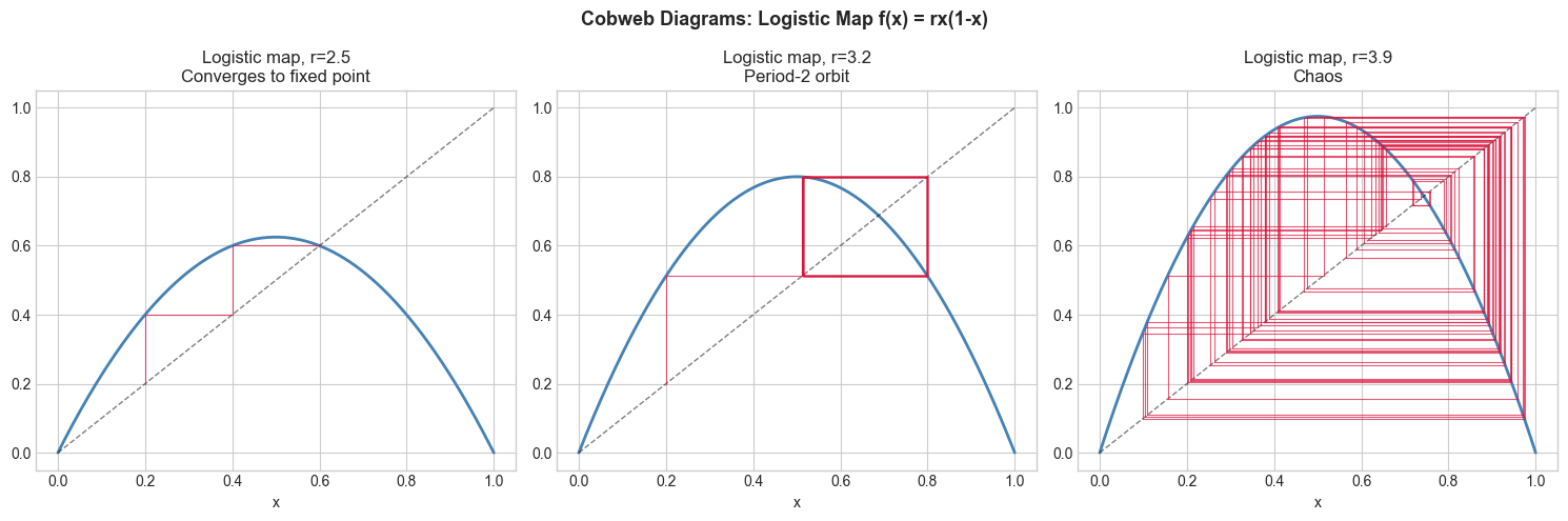
5. Python Implementation
# --- Implementation: Discrete dynamical system simulator ---
import numpy as np

def simulate_dynamical_system(f, x0, n_steps):
    """
    Simulate the dynamical system xₙ₊₁ = f(xₙ).

    Args:
        f: callable, the update rule
        x0: initial state (scalar or array)
        n_steps: int, number of iterations
    Returns:
        np.ndarray of shape (n_steps+1, ...) containing the orbit
    """
    x0 = np.asarray(x0, dtype=float)
    orbit = [x0]
    x = x0.copy()
    for _ in range(n_steps):
        x = f(x)
        orbit.append(x.copy())
    return np.array(orbit)

def find_fixed_points(f, x_grid, tol=1e-6):
    """Find approximate fixed points by locating where f(x) ≈ x."""
    diff = f(x_grid) - x_grid
    sign_changes = np.where(np.diff(np.sign(diff)))[0]
    return x_grid[sign_changes]

# Logistic map analysis
R_VALUES = [1.5, 2.5, 3.2, 3.5, 3.9]
print("Logistic map long-term behavior:")
for r in R_VALUES:
    f = lambda x, r=r: r*x*(1-x)
    orbit = simulate_dynamical_system(f, 0.3, 500)
    tail = orbit[-50:]  # last 50 steps (after transient)
    unique_vals = np.unique(tail.round(4))
    if len(unique_vals) <= 4:
        print(f"  r={r}: attractor at {unique_vals}")
    else:
        print(f"  r={r}: chaos ({len(unique_vals)} unique values in last 50 steps)")
Logistic map long-term behavior:
r=1.5: attractor at [0.3333]
r=2.5: attractor at [0.6]
r=3.2: attractor at [0.513 0.7995]
r=3.5: attractor at [0.3828 0.5009 0.8269 0.875 ]
r=3.9: chaos (49 unique values in last 50 steps)
6. Experiments
Experiment 1: Run the logistic map for r from 2 to 4 in steps of 0.01. Plot the long-term behavior (orbit tail) as a bifurcation diagram. This is one of the most famous pictures in mathematics.
Experiment 2: Simulate a 2D system: xₙ₊₁ = r·xₙ·(1-xₙ-αyₙ), yₙ₊₁ = s·yₙ·(1-yₙ-βxₙ). This is a competitive Lotka-Volterra model. Vary α and β and observe coexistence vs extinction.
7. Exercises
Easy 1. The map xₙ₊₁ = 0.9·xₙ + 1 has a fixed point. Find it analytically and verify by simulating.
Easy 2. Simulate xₙ₊₁ = cos(xₙ) starting at x₀=1 for 100 steps. What value does it converge to? This is the Dottie number.
Medium 1. Implement a bifurcation diagram for the logistic map: for each r in [2.5, 4.0], simulate 500 steps, discard first 400, plot the last 100. Plot all (r, x) pairs together.
Medium 2. For the logistic map with r=3.9, show sensitive dependence: simulate two orbits starting at x₀=0.500 and x₀=0.501. Plot |difference| vs time on a log scale.
Hard. Implement the Lyapunov exponent for a 1D map: λ = lim_{n→∞} (1/n) Σᵢ log|f’(xᵢ)|. For the logistic map, compute λ for r from 2 to 4. λ > 0 indicates chaos. Verify your bifurcation diagram and Lyapunov exponent match.
9. Chapter Summary & Connections
Discrete dynamical systems: xₙ₊₁ = f(xₙ) — the orbit is the sequence of states
Fixed points: f(x*)=x*; stable if |f’(x*)| < 1
Logistic map exhibits period doubling, chaos, sensitive dependence
Machine learning training is a dynamical system on parameter space
Forward connections:
ch077 (Chaos) deepens the analysis with Lyapunov exponents and bifurcation diagrams
ch082 (Predator-Prey Project) uses 2D discrete dynamical systems
AR(1) time series models in ch285 are linear discrete dynamical systems