Chapter 124 — Vector Representation - Mathematics for Programmers

Prerequisites: Vectors in Programming (ch123), Geometric Interpretation (ch122), trigonometry (ch101–103) You will learn:
Cartesian representation vs polar representation
Column vectors vs row vectors — and why the distinction matters
Converting between representations
How high-dimensional vectors are represented even when they cannot be drawn

Environment: Python 3.x, numpy, matplotlib

1. Concept¶

A vector is an abstract object. To work with it computationally, we need a representation: a way of writing the vector as an ordered collection of numbers.

The most common representation is Cartesian coordinates — the components along each axis. But there are others. In 2D, a vector can also be represented as (magnitude, angle) — the polar form. Both representations encode the same vector.

A second dimension of representation choice: column vector vs row vector.

\text{Column: } \mathbf{v} = \begin{pmatrix} 1 \\ 2 \\ 3 \end{pmatrix} \qquad \text{Row: } \mathbf{v}^T = \begin{pmatrix} 1 & 2 & 3 \end{pmatrix}

(1)

Mathematically, these are different objects (a column vector has shape n×1, a row vector has shape 1×n). In NumPy, a 1D array np.array([1, 2, 3]) has shape (3,) and is neither — it becomes column or row depending on context. This is the source of many subtle bugs.

Common misconception: A NumPy 1D array shape=(n,) is not the same as a column vector shape=(n,1) or a row vector shape=(1,n). Operations like matrix multiplication will behave differently.

2. Intuition & Mental Models¶

Polar model: Think of any 2D vector as an arm of a clock. The length of the arm is the magnitude. The angle it makes with the positive x-axis is the direction. These two numbers — length and angle — determine the arm completely.

Coordinate model: Think of the same arm as a staircase: walk some distance right (x-component), then some distance up (y-component). The staircase has the same net effect as the arm.

Column vs row: By mathematical convention (and ML convention), vectors are columns — vertical lists. Row vectors are their transposes. In NumPy, always prefer shape (n,) for standalone vectors, and be explicit about shape when doing matrix operations.

Recall from ch101–103 (Trigonometry, Sine and Cosine, Unit Circle) that $x = r\cos\theta$ and $y = r\sin\theta$ give the Cartesian components from polar.

3. Visualization¶

# --- Visualization: Cartesian vs polar representation ---
import numpy as np
import matplotlib.pyplot as plt
plt.style.use('seaborn-v0_8-whitegrid')

# Define a vector in polar: magnitude r, angle theta (radians)
r     = 3.0
theta = np.pi / 4   # 45 degrees

# Convert to Cartesian
x = r * np.cos(theta)
y = r * np.sin(theta)

fig, axes = plt.subplots(1, 2, figsize=(12, 5))

# ---- Left: Cartesian ----
ax = axes[0]
ax.annotate('', xy=(x, y), xytext=(0, 0),
            arrowprops=dict(arrowstyle='->', color='steelblue', lw=2.5))
ax.plot([0, x], [0, 0], 'k--', lw=1, label=f'x = {x:.2f}')
ax.plot([x, x], [0, y], 'k:',  lw=1, label=f'y = {y:.2f}')
ax.text(x+0.05, y+0.05, f'v=({x:.2f}, {y:.2f})', fontsize=11, color='steelblue')
ax.set_xlim(-0.5, 4); ax.set_ylim(-0.5, 4)
ax.axhline(0, color='black', lw=0.7); ax.axvline(0, color='black', lw=0.7)
ax.set_aspect('equal')
ax.set_title('Cartesian Representation')
ax.set_xlabel('x'); ax.set_ylabel('y')
ax.legend()

# ---- Right: Polar ----
ax = axes[1]
ax.annotate('', xy=(x, y), xytext=(0, 0),
            arrowprops=dict(arrowstyle='->', color='coral', lw=2.5))
# Draw arc for angle
arc_angles = np.linspace(0, theta, 50)
ARC_R = 0.8
ax.plot(ARC_R * np.cos(arc_angles), ARC_R * np.sin(arc_angles), 'k-', lw=1.5)
ax.text(ARC_R*1.1*np.cos(theta/2), ARC_R*1.1*np.sin(theta/2),
        f'θ={np.degrees(theta):.0f}°', fontsize=11)
# Label magnitude
mid = np.array([x/2, y/2])
ax.text(mid[0]+0.1, mid[1]+0.1, f'r={r:.1f}', fontsize=11, color='coral')
ax.set_xlim(-0.5, 4); ax.set_ylim(-0.5, 4)
ax.axhline(0, color='black', lw=0.7); ax.axvline(0, color='black', lw=0.7)
ax.set_aspect('equal')
ax.set_title('Polar Representation')
ax.set_xlabel('x'); ax.set_ylabel('y')

plt.tight_layout()
plt.show()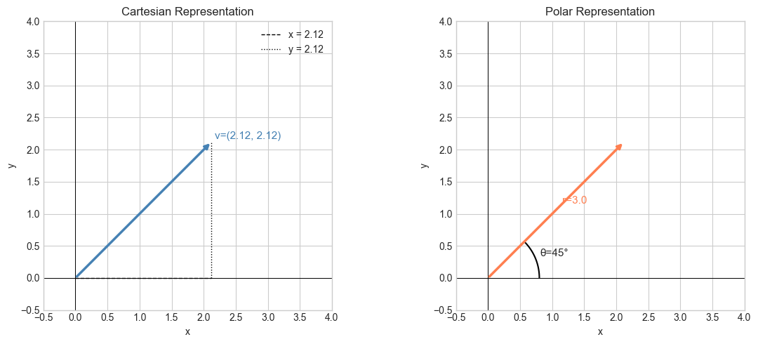

4. Mathematical Formulation¶

Cartesian to Polar (2D):

r = \|\mathbf{v}\| = \sqrt{v_x^2 + v_y^2}

(2)

\theta = \text{atan2}(v_y, v_x)

(3)

Where:

$r$ = magnitude (length) of the vector
$\theta$ = angle from positive x-axis (in radians)
atan2 is used instead of atan to handle all four quadrants correctly

Polar to Cartesian:

v_x = r \cos\theta \qquad v_y = r \sin\theta

(4)

Column vs row in NumPy shapes:

v      = np.array([1, 2, 3])     # shape (3,)  — "flat" vector
v_col  = v.reshape(-1, 1)        # shape (3,1) — column vector
v_row  = v.reshape(1, -1)        # shape (1,3) — row vector

# --- Mathematical Formulation: conversion functions ---
import numpy as np

def cartesian_to_polar(v):
    """
    Convert 2D Cartesian vector to polar (r, theta).

    Args:
        v: ndarray shape (2,)

    Returns:
        (r, theta) where r >= 0 and theta in (-pi, pi]
    """
    r = np.linalg.norm(v)
    theta = np.arctan2(v[1], v[0])  # atan2 handles all quadrants
    return r, theta


def polar_to_cartesian(r, theta):
    """
    Convert polar (r, theta) to 2D Cartesian vector.

    Args:
        r: float, magnitude >= 0
        theta: float, angle in radians

    Returns:
        ndarray shape (2,)
    """
    return np.array([r * np.cos(theta), r * np.sin(theta)])


# Test round-trip
for v in [np.array([3.0, 0.0]), np.array([0.0, 2.0]),
          np.array([-1.0, 1.0]), np.array([3.0, -4.0])]:
    r, theta = cartesian_to_polar(v)
    v_back = polar_to_cartesian(r, theta)
    err = np.linalg.norm(v - v_back)
    print(f"v={v}  r={r:.3f}  theta={np.degrees(theta):.1f}°  round-trip error={err:.2e}")

v=[3. 0.]  r=3.000  theta=0.0°  round-trip error=0.00e+00
v=[0. 2.]  r=2.000  theta=90.0°  round-trip error=1.22e-16
v=[-1.  1.]  r=1.414  theta=135.0°  round-trip error=2.22e-16
v=[ 3. -4.]  r=5.000  theta=-53.1°  round-trip error=6.28e-16

5. Python Implementation¶

# --- Implementation: Shape handling for column/row vectors ---
import numpy as np

def as_column(v):
    """
    Return v as a column vector with shape (n, 1).

    Args:
        v: ndarray shape (n,) or (n,1)

    Returns:
        ndarray shape (n,1)
    """
    v = np.asarray(v, dtype=float)
    return v.reshape(-1, 1)


def as_row(v):
    """
    Return v as a row vector with shape (1, n).

    Args:
        v: ndarray shape (n,) or (n,1)

    Returns:
        ndarray shape (1,n)
    """
    v = np.asarray(v, dtype=float)
    return v.reshape(1, -1)


def as_flat(v):
    """
    Return v as a flat vector with shape (n,).

    Args:
        v: ndarray of any compatible shape

    Returns:
        ndarray shape (n,)
    """
    return np.asarray(v, dtype=float).flatten()


v = np.array([1.0, 2.0, 3.0])
print("Flat   shape:", as_flat(v).shape)
print("Column shape:", as_column(v).shape)
print("Row    shape:", as_row(v).shape)
print()
print("Column vector:\n", as_column(v))
print("Row vector:\n", as_row(v))

Flat   shape: (3,)
Column shape: (3, 1)
Row    shape: (1, 3)

Column vector:
 [[1.]
 [2.]
 [3.]]
Row vector:
 [[1. 2. 3.]]

6. Experiments¶

# --- Experiment 1: Quadrant behavior of atan2 ---
# Hypothesis: atan2 correctly identifies angle for all four quadrants.
# Try changing: the vector components to explore each quadrant.
import numpy as np

VECTORS = [
    np.array([ 1.0,  0.0]),   # East — 0°
    np.array([ 0.0,  1.0]),   # North — 90°
    np.array([-1.0,  0.0]),   # West — 180°
    np.array([ 0.0, -1.0]),   # South — -90°
    np.array([-1.0, -1.0]),   # SW  — modify this
]

for v in VECTORS:
    theta_rad = np.arctan2(v[1], v[0])
    theta_deg = np.degrees(theta_rad)
    print(f"v={v}  theta={theta_deg:7.2f}°")

v=[1. 0.]  theta=   0.00°
v=[0. 1.]  theta=  90.00°
v=[-1.  0.]  theta= 180.00°
v=[ 0. -1.]  theta= -90.00°
v=[-1. -1.]  theta=-135.00°

# --- Experiment 2: Shape gotchas in NumPy ---
# Hypothesis: operations between (3,) and (3,1) arrays behave differently than expected.
# Try changing: the shapes and observe the output shape.
import numpy as np

v_flat = np.array([1.0, 2.0, 3.0])         # shape (3,)
v_col  = np.array([[1.0], [2.0], [3.0]])    # shape (3,1)
v_row  = np.array([[1.0, 2.0, 3.0]])        # shape (1,3)

print("Shapes:", v_flat.shape, v_col.shape, v_row.shape)
print()

# What shape does multiplication produce?
print("flat * flat:", (v_flat * v_flat).shape)   # (3,)
print("col * row:  ", (v_col  * v_row).shape)     # (3,3) — outer product!
print("row * col:  ", (v_row  * v_col).shape)     # (3,3)
print("flat * col: ", (v_flat * v_col).shape)     # broadcasts to (3,3)

Shapes: (3,) (3, 1) (1, 3)

flat * flat: (3,)
col * row:   (3, 3)
row * col:   (3, 3)
flat * col:  (3, 3)

7. Exercises¶

Easy 1. Convert the vector v = (3, 4) from Cartesian to polar. What is its magnitude? What angle does it make with the x-axis? (Expected: r=5, theta≈53.13°)

Easy 2. Convert polar (r=2, theta=120°) to Cartesian. (Expected: (-1, 1.732))

Medium 1. Write a function polar_to_cartesian_batch(rs, thetas) that converts arrays of radii and angles to an array of Cartesian vectors. Shape of output: (n, 2). Test with 5 vectors.

Medium 2. Create a 4D vector v = (1, 2, 3, 4). Reshape it as a column vector (4, 1) and a row vector (1, 4). Multiply column by row — what shape is the result? What is the result’s entry at position (i, j)? (Hint: outer product — connects to ch131)

Hard. The angle theta from atan2 lies in (-π, π]. Write a function normalize_angle(theta) that converts any angle to [0, 2π). Verify that cartesian_to_polar → polar_to_cartesian is a perfect round-trip for 100 random vectors. What precision do you observe?

8. Mini Project¶

# --- Mini Project: Radar Display ---
# Problem: A radar system tracks objects using polar coordinates (range, bearing).
#          Convert to Cartesian and display on a 2D grid.
# Dataset: simulated radar returns
# Task: implement conversion, filter objects within a safe zone, display results

import numpy as np
import matplotlib.pyplot as plt
plt.style.use('seaborn-v0_8-whitegrid')

# Radar returns: (range_km, bearing_degrees clockwise from North)
# North is +y in Cartesian coordinates
radar_returns = np.array([
    [5.2,  30],
    [8.1,  120],
    [3.0,  200],
    [10.5, 315],
    [6.7,  45],
    [2.1,  90],
    [9.0,  270],
    [4.4,  160],
])

SAFE_ZONE_RADIUS = 5.0  # km — objects within this are a concern

def radar_to_cartesian(range_km, bearing_deg):
    """
    Convert radar polar coordinates to Cartesian (x=East, y=North).

    Args:
        range_km: float
        bearing_deg: float, degrees clockwise from North

    Returns:
        (x, y): tuple of floats
    """
    # TODO: implement (North = +y, clockwise bearing)
    pass

# TODO: convert all returns, identify those within safe zone radius, visualize

9. Summary & Connections¶

Cartesian representation: components along each axis — the standard for computation.
Polar representation: magnitude and angle — natural for rotation and direction problems.
Column vs row vs flat: shape matters for matrix multiplication. Default to (n,) unless doing matrix algebra.
np.arctan2(y, x) handles all quadrants correctly; np.arctan(y/x) does not.

Backward connection: This applies the unit circle and trigonometry from ch103. The polar-to-Cartesian formula $x = r\cos\theta$ , $y = r\sin\theta$ is directly the unit circle definition.

Forward connections:

This will reappear in ch128 — Vector Length (Norm), where the Cartesian-to-polar radius formula becomes the Euclidean norm.
This will reappear in ch133 — Angles Between Vectors, where the angle between two vectors is computed without converting to polar.
This will reappear in ch151 — Introduction to Matrices (Part VI), where column vectors are the standard input/output type for matrix multiplication.