Prerequisites: ch131 (dot product), ch135 (orthogonality), ch121 (vectors)
You will learn:
What the cross product is and when it is defined
How to compute it and what its direction and magnitude mean
Why the cross product measures oriented area
Applications in 3D graphics, physics, and computational geometry
Environment: Python 3.x, numpy, matplotlib
1. Concept
The cross product takes two 3D vectors and returns a third vector that is perpendicular to both:
The cross product is defined only in 3D (and in 7D, a generalization that is rarely needed). In 2D, there is no vector orthogonal to two given vectors — you can compute a scalar “2D cross product” (the -component only), but it is not a full vector.
Common misconceptions:
The cross product is not commutative: .
The cross product of parallel vectors is the zero vector (they span no area).
The cross product does not generalize to dimensions in the same way the dot product does.
2. Intuition & Mental Models
Geometric: Place your right hand so your fingers curl from toward . Your thumb points in the direction of . This is the right-hand rule — it encodes orientation.
Area: The magnitude equals the area of the parallelogram spanned by and :
When and are parallel (), the area is zero and so is the cross product.
Computational (3D graphics): Surface normals in 3D meshes are computed via cross products. Two edges of a triangle give two vectors; their cross product gives the direction the surface faces. Every lighting calculation in graphics depends on this.
Contrast with dot product: The dot product measures parallel alignment (cosine of angle). The cross product measures perpendicular extent (sine of angle). Together they decompose the full geometric relationship between two vectors.
Recall from ch135: the cross product vector is orthogonal to both inputs — its dot product with either or is zero.
3. Visualization
# --- Visualization: Cross product as perpendicular vector ---

import numpy as np
import matplotlib.pyplot as plt
from mpl_toolkits.mplot3d import Axes3D

plt.style.use('seaborn-v0_8-whitegrid')

a = np.array([2.0, 0.0, 0.0])
b = np.array([0.5, 1.5, 0.0])
c = np.cross(a, b)

fig = plt.figure(figsize=(12, 5))

# 3D view
ax3d = fig.add_subplot(121, projection='3d')
ORIGIN = np.zeros(3)
ax3d.quiver(*ORIGIN, *a, color='steelblue', linewidth=2, label=f'a={a}')
ax3d.quiver(*ORIGIN, *b, color='tomato',    linewidth=2, label=f'b={b}')
ax3d.quiver(*ORIGIN, *c, color='seagreen',  linewidth=2, label=f'a×b={np.round(c,2)}')

# Draw parallelogram
corners = np.array([ORIGIN, a, a+b, b, ORIGIN])
ax3d.plot(corners[:,0], corners[:,1], corners[:,2], 'gray', alpha=0.4, linestyle='--')

ax3d.set_xlim(0, 2.5); ax3d.set_ylim(0, 2); ax3d.set_zlim(0, 3.5)
ax3d.set_xlabel('x'); ax3d.set_ylabel('y'); ax3d.set_zlabel('z')
ax3d.set_title(f'a×b perpendicular to both\n||a×b|| = {np.linalg.norm(c):.3f} (parallelogram area)')
ax3d.legend(fontsize=8)

# Angle sweep: |a×b| = ||a|| ||b|| sin(θ)
ax2 = fig.add_subplot(122)
thetas = np.linspace(0, np.pi, 200)
norm_a, norm_b = 2.0, 1.5
cross_mags = norm_a * norm_b * np.sin(thetas)
dot_prods   = norm_a * norm_b * np.cos(thetas)

ax2.plot(np.degrees(thetas), cross_mags, 'seagreen', linewidth=2, label='||a×b|| = ||a||||b||sinθ')
ax2.plot(np.degrees(thetas), dot_prods,  'steelblue', linewidth=2, linestyle='--', label='a·b = ||a||||b||cosθ')
ax2.axhline(0, color='gray', linewidth=0.8)
ax2.set_xlabel('Angle θ (degrees)')
ax2.set_ylabel('Value')
ax2.set_title('Cross Product Magnitude vs Dot Product vs Angle')
ax2.legend(fontsize=9)

plt.tight_layout()
plt.show()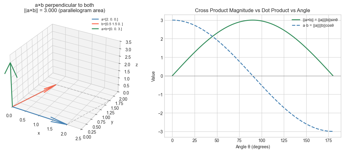
4. Mathematical Formulation
Component formula:
Properties:
Anti-commutativity:
Bilinearity: ;
Zero for parallels:
Orthogonality: and
Magnitude:
This is the area of the parallelogram spanned by and .
Triple product (scalar): The signed volume of the parallelepiped spanned by three vectors:
If , the three vectors are coplanar (linearly dependent). (This connects to ch158 — Determinants, which generalizes signed volume.)
5. Python Implementation
# --- Implementation: cross product from scratch ---

def cross_product(a, b):
    """
    3D cross product.

    Args:
        a, b: array-like, shape (3,)

    Returns:
        array, shape (3,): vector perpendicular to both a and b

    Raises:
        ValueError: if inputs are not 3D
    """
    a, b = np.asarray(a, float), np.asarray(b, float)
    if a.shape != (3,) or b.shape != (3,):
        raise ValueError(f"Cross product requires 3D vectors, got {a.shape} and {b.shape}")
    return np.array([
        a[1]*b[2] - a[2]*b[1],
        a[2]*b[0] - a[0]*b[2],
        a[0]*b[1] - a[1]*b[0],
    ])


def parallelogram_area(a, b):
    """Area of parallelogram spanned by a and b."""
    return np.linalg.norm(cross_product(a, b))


def triangle_area(p1, p2, p3):
    """Area of triangle with vertices p1, p2, p3 in 3D."""
    v1 = np.asarray(p2) - np.asarray(p1)
    v2 = np.asarray(p3) - np.asarray(p1)
    return 0.5 * parallelogram_area(v1, v2)


def triple_product(a, b, c):
    """Scalar triple product = a · (b × c) = signed volume."""
    return np.dot(np.asarray(a), cross_product(b, c))


def surface_normal(p1, p2, p3):
    """Unit normal vector of a triangle (for 3D graphics)."""
    v1 = np.asarray(p2, float) - np.asarray(p1, float)
    v2 = np.asarray(p3, float) - np.asarray(p1, float)
    n = cross_product(v1, v2)
    return n / np.linalg.norm(n)


# Tests
a = np.array([1.0, 0.0, 0.0])
b = np.array([0.0, 1.0, 0.0])
c = cross_product(a, b)
print(f"e1 × e2 = {c}  (expect [0, 0, 1])")
print(f"e2 × e1 = {cross_product(b, a)}  (expect [0, 0, -1])  — anti-commutative")

print(f"\nOrthogonality check: a·(a×b) = {np.dot(a, c):.2e}")
print(f"Orthogonality check: b·(a×b) = {np.dot(b, c):.2e}")

# Triangle area
p1 = np.array([0.0, 0.0, 0.0])
p2 = np.array([1.0, 0.0, 0.0])
p3 = np.array([0.0, 1.0, 0.0])
print(f"\nTriangle area: {triangle_area(p1, p2, p3):.4f}  (expect 0.5)")

# Validate against numpy
a_rand = np.random.randn(3)
b_rand = np.random.randn(3)
assert np.allclose(cross_product(a_rand, b_rand), np.cross(a_rand, b_rand))
print("Validation against np.cross: PASSED")
e1 × e2 = [0. 0. 1.] (expect [0, 0, 1])
e2 × e1 = [ 0. 0. -1.] (expect [0, 0, -1]) — anti-commutative
Orthogonality check: a·(a×b) = 0.00e+00
Orthogonality check: b·(a×b) = 0.00e+00
Triangle area: 0.5000 (expect 0.5)
Validation against np.cross: PASSED
6. Experiments
# --- Experiment 1: Anti-commutativity and its geometric meaning ---
# Hypothesis: a×b and b×a have the same magnitude but opposite directions.
# Swapping the input order flips the surface normal.

a = np.array([1.0, 2.0, 0.5])
b = np.array([0.5, 1.0, 2.0])

axb = cross_product(a, b)
bxa = cross_product(b, a)

print(f"a × b = {np.round(axb, 3)}")
print(f"b × a = {np.round(bxa, 3)}")
print(f"Sum:   {np.round(axb + bxa, 10)}  (should be zero)")
print(f"||a×b|| = ||b×a|| = {np.linalg.norm(axb):.4f}")
a × b = [ 3.5 -1.75 0. ]
b × a = [-3.5 1.75 0. ]
Sum: [0. 0. 0.] (should be zero)
||a×b|| = ||b×a|| = 3.9131
# --- Experiment 2: Area computation via cross product ---
# Hypothesis: splitting a polygon into triangles and summing areas
# gives the correct total area.
# Try changing: RADIUS and N_SIDES

N_SIDES = 6    # <-- modify this
RADIUS  = 2.0  # <-- modify this

# Regular polygon vertices in XY plane (z = 0)
angles = np.linspace(0, 2*np.pi, N_SIDES, endpoint=False)
vertices = np.column_stack([
    RADIUS * np.cos(angles),
    RADIUS * np.sin(angles),
    np.zeros(N_SIDES)
])

center = np.zeros(3)
total_area = sum(
    triangle_area(center, vertices[i], vertices[(i+1) % N_SIDES])
    for i in range(N_SIDES)
)

# Analytical area of regular polygon
true_area = 0.5 * N_SIDES * RADIUS**2 * np.sin(2*np.pi/N_SIDES)

print(f"N_SIDES = {N_SIDES}, RADIUS = {RADIUS}")
print(f"Cross-product area: {total_area:.6f}")
print(f"Analytical area:    {true_area:.6f}")
print(f"Error: {abs(total_area - true_area):.2e}")
print(f"\n(As N_SIDES → ∞, the polygon approaches a circle with area π*R² = {np.pi*RADIUS**2:.4f})")
N_SIDES = 6, RADIUS = 2.0
Cross-product area: 10.392305
Analytical area: 10.392305
Error: 0.00e+00
(As N_SIDES → ∞, the polygon approaches a circle with area π*R² = 12.5664)
# --- Experiment 3: Surface normals in a simple 3D mesh ---
# Compute and display surface normals for a set of triangles.
# Try changing: the vertex positions.

# A simple "tent" shape: 4 triangles
apex   = np.array([0.0, 0.0, 2.0])  # <-- modify this
p1 = np.array([-1.0, -1.0, 0.0])
p2 = np.array([ 1.0, -1.0, 0.0])
p3 = np.array([ 1.0,  1.0, 0.0])
p4 = np.array([-1.0,  1.0, 0.0])

triangles = [(p1, p2, apex), (p2, p3, apex), (p3, p4, apex), (p4, p1, apex)]

fig = plt.figure(figsize=(8, 6))
ax = fig.add_subplot(111, projection='3d')

COLORS = ['steelblue', 'tomato', 'seagreen', 'orange']
for (t1, t2, t3), color in zip(triangles, COLORS):
    n = surface_normal(t1, t2, t3)
    centroid = (t1 + t2 + t3) / 3
    # Draw triangle edges
    tri = np.array([t1, t2, t3, t1])
    ax.plot(tri[:,0], tri[:,1], tri[:,2], color=color, linewidth=1)
    # Draw normal at centroid
    ax.quiver(*centroid, *n*0.5, color=color, linewidth=2)

ax.set_xlabel('x'); ax.set_ylabel('y'); ax.set_zlabel('z')
ax.set_title('Surface Normals via Cross Product')
plt.tight_layout()
plt.show()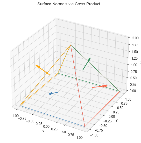
7. Exercises
Easy 1. Compute by hand using the formula, then verify with np.cross. (Expected: )
Easy 2. What is for any vector ? Why? (Expected: the zero vector — prove using the formula)
Medium 1. Given three points , , , find the equation of the plane through them. (Hint: the surface normal gives the plane’s coefficients )
Medium 2. Verify the Jacobi identity numerically: . Test on 10 random triples.
Hard. The vector triple product satisfies (the BAC-CAB rule). Prove this algebraically by expanding both sides in components. Then verify numerically.
8. Mini Project — 3D Mesh Normal Smoothing
# --- Mini Project: Surface Normal Computation for a Sphere Mesh ---
# Problem: Approximate a sphere with triangulated faces.
#          Compute per-face surface normals using the cross product.
# Dataset: Parametric sphere mesh generated here.
# Task: Complete compute_face_normals and visualize with quiver plot.

def generate_sphere_mesh(n_lat=8, n_lon=8, radius=1.0):
    """
    Generate triangle faces of a sphere.

    Returns:
        faces: list of (p1, p2, p3) triangles, each vertex is shape (3,)
    """
    lats = np.linspace(0, np.pi, n_lat + 1)
    lons = np.linspace(0, 2*np.pi, n_lon + 1)

    def to_xyz(lat, lon):
        return radius * np.array([np.sin(lat)*np.cos(lon),
                                   np.sin(lat)*np.sin(lon),
                                   np.cos(lat)])

    faces = []
    for i in range(n_lat):
        for j in range(n_lon):
            p00 = to_xyz(lats[i],   lons[j])
            p10 = to_xyz(lats[i+1], lons[j])
            p01 = to_xyz(lats[i],   lons[j+1])
            p11 = to_xyz(lats[i+1], lons[j+1])
            faces.append((p00, p10, p11))
            faces.append((p00, p11, p01))
    return faces


def compute_face_normals(faces):
    """
    Compute unit normal for each triangular face.

    Args:
        faces: list of (p1, p2, p3) triangles

    Returns:
        centroids: array (n_faces, 3)
        normals:   array (n_faces, 3), unit normals
    """
    centroids = []
    normals   = []
    for p1, p2, p3 in faces:
        # TODO: compute centroid
        centroid = None  # replace
        # TODO: compute unit normal via cross product
        normal = None    # replace
        centroids.append(centroid)
        normals.append(normal)
    return np.array(centroids), np.array(normals)


# --- Test (uncomment after implementing) ---
# faces = generate_sphere_mesh(n_lat=6, n_lon=6)
# centroids, normals = compute_face_normals(faces)
#
# fig = plt.figure(figsize=(8, 8))
# ax = fig.add_subplot(111, projection='3d')
# ax.quiver(centroids[:,0], centroids[:,1], centroids[:,2],
#            normals[:,0],   normals[:,1],   normals[:,2],
#            length=0.15, color='tomato', alpha=0.7)
# ax.set_title('Surface Normals on Sphere Mesh')
# ax.set_xlabel('x'); ax.set_ylabel('y'); ax.set_zlabel('z')
# plt.tight_layout()
# plt.show()
#
# # Verification: for a unit sphere, the normal at any surface point
# # should equal the position vector itself.
# dot_check = np.sum(centroids * normals, axis=1)
# print(f"Normal · centroid (should be ~1.0): min={dot_check.min():.4f}, max={dot_check.max():.4f}")
9. Chapter Summary & Connections
The cross product is a vector perpendicular to both and , defined only in 3D.
Its magnitude gives the area of the parallelogram they span.
It is anti-commutative: — order matters and encodes orientation.
The scalar triple product gives signed volume and detects coplanarity.
Forward connections:
This reappears in ch158 — Determinants, where the 3×3 determinant equals the scalar triple product — generalizing signed volume to dimensions.
This reappears in ch149 — Project: Particle Simulation, where cross products compute torque and angular momentum.
This is the foundation of surface rendering in ch115 — Computer Graphics Basics.
Backward connection:
This builds on ch135 — Orthogonality: the result is perpendicular to both inputs by construction, verified by .
Going deeper: The cross product is a special case of the exterior product (wedge product) in differential geometry. The exterior product generalizes to any dimension and underlies differential forms, Stokes’ theorem, and manifold theory.