Prerequisites: ch154 (matrix multiplication), ch164 (linear transformations), ch168 (projection matrices), ch176 (matrix calculus) You will learn:
How a neural network forward pass is a sequence of matrix multiplications
What role weight matrices and bias vectors play geometrically
How activation functions break linearity — and why that matters
How matrix shapes propagate through a network
Why the chain rule from ch176 is the engine of backpropagation
Environment: Python 3.x, numpy, matplotlib
1. Concept
A neural network, stripped of its mystique, is a composition of affine transformations interleaved with nonlinearities.
Each layer computes:
output = activation(W @ input + b)Where W is a weight matrix, b is a bias vector, and activation is a nonlinear function applied elementwise.
Everything before the activation is pure linear algebra — the same linear algebra from ch151–ch176. The activation function is the only ingredient that was not in those chapters.
What problem does this solve?
Without matrix algebra, we could not efficiently describe transformations of high-dimensional data. A single fully-connected layer mapping 784 inputs (a 28×28 image) to 256 hidden units requires 784×256 = 200,704 scalar multiplications. Matrix notation compresses this into one line: h = W @ x + b.
Common misconception: Neural networks are not doing something fundamentally different from linear algebra. They are doing a lot of it, composed deeply, with nonlinearities inserted at each layer to prevent the whole stack from collapsing into a single matrix.
2. Intuition & Mental Models
Geometric analogy: Think of each layer as a coordinate transformation. The weight matrix rotates, scales, and shears the input space. The bias shifts it. The activation then folds the space — introducing curvature that no single linear transformation could produce. Stack enough of these fold-and-transform operations and you can represent arbitrarily complex boundaries.
Computational analogy: Think of a neural network as a function factory. Each layer is a parameterized function f_i(x) = σ(W_i @ x + b_i). The network is f_L ∘ f_{L-1} ∘ ... ∘ f_1. The parameters (W_i, b_i) are what training adjusts.
Why linearity alone fails: Recall from ch164 that linear transformations map lines to lines. No matter how many you stack, the composition is still linear — a single matrix. You cannot learn XOR (a nonlinearly separable problem) with any number of purely linear layers. Activations are what break this constraint.
Shape arithmetic is everything: If x has shape (n,) and you want output of shape (m,), then W must be (m, n) and b must be (m,). Getting shapes wrong is the most common implementation error. Every layer’s output becomes the next layer’s input — the shapes must chain.
3. Visualization
# --- Visualization: How layers transform a 2D point cloud ---
import numpy as np
import matplotlib.pyplot as plt
plt.style.use('seaborn-v0_8-whitegrid')

np.random.seed(42)

# Generate two classes of 2D points
N = 80
class0 = np.random.randn(N, 2) * 0.4 + np.array([1, 1])
class1 = np.random.randn(N, 2) * 0.4 + np.array([-1, -1])
X = np.vstack([class0, class1])          # (160, 2)
labels = np.array([0]*N + [1]*N)

# Layer 1: W1 (3x2), b1 (3,) — maps R^2 -> R^3
W1 = np.array([[1.2, -0.5],
               [0.3,  1.1],
               [-0.8, 0.6]])
b1 = np.array([0.1, -0.2, 0.3])

def relu(z):
    return np.maximum(0, z)

# Forward through layer 1
Z1 = X @ W1.T + b1     # (160, 3)
H1 = relu(Z1)          # (160, 3) — nonlinearity applied

fig, axes = plt.subplots(1, 3, figsize=(14, 4))

colors = ['steelblue' if l == 0 else 'tomato' for l in labels]

# Input space
axes[0].scatter(X[:, 0], X[:, 1], c=colors, alpha=0.6, s=20)
axes[0].set_title('Input Space (R²)', fontsize=12)
axes[0].set_xlabel('x₁'); axes[0].set_ylabel('x₂')

# After linear transform (pre-activation)
axes[1].scatter(Z1[:, 0], Z1[:, 1], c=colors, alpha=0.6, s=20)
axes[1].set_title('After Linear Transform (pre-ReLU)', fontsize=12)
axes[1].set_xlabel('z₁'); axes[1].set_ylabel('z₂')

# After ReLU
axes[2].scatter(H1[:, 0], H1[:, 1], c=colors, alpha=0.6, s=20)
axes[2].set_title('After ReLU (hidden representation)', fontsize=12)
axes[2].set_xlabel('h₁'); axes[2].set_ylabel('h₂')

plt.suptitle('2D Input → Linear Transform → ReLU: Classes Separating', fontsize=13)
plt.tight_layout()
plt.show()
print(f"Input shape: {X.shape}")
print(f"W1 shape: {W1.shape}  — maps R^2 -> R^3")
print(f"Z1 shape: {Z1.shape}  — after linear transform")
print(f"H1 shape: {H1.shape}  — after ReLU")
C:\Users\user\AppData\Local\Temp\ipykernel_2856\2084897196.py:48: UserWarning: Glyph 8321 (\N{SUBSCRIPT ONE}) missing from font(s) Arial.
plt.tight_layout()
C:\Users\user\AppData\Local\Temp\ipykernel_2856\2084897196.py:48: UserWarning: Glyph 8322 (\N{SUBSCRIPT TWO}) missing from font(s) Arial.
plt.tight_layout()
c:\Users\user\OneDrive\Documents\book\.venv\Lib\site-packages\IPython\core\pylabtools.py:170: UserWarning: Glyph 8322 (\N{SUBSCRIPT TWO}) missing from font(s) Arial.
fig.canvas.print_figure(bytes_io, **kw)
c:\Users\user\OneDrive\Documents\book\.venv\Lib\site-packages\IPython\core\pylabtools.py:170: UserWarning: Glyph 8321 (\N{SUBSCRIPT ONE}) missing from font(s) Arial.
fig.canvas.print_figure(bytes_io, **kw)
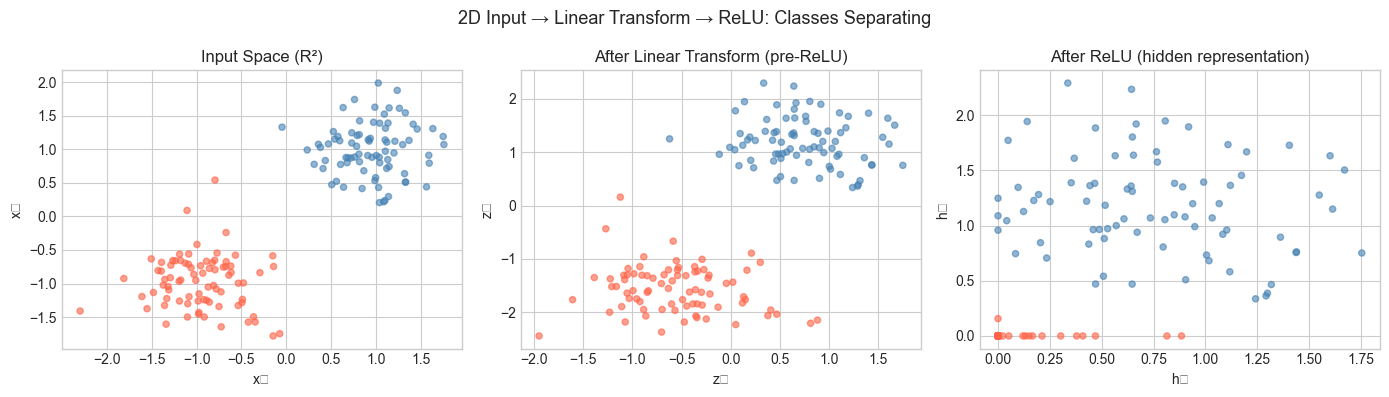
Input shape: (160, 2)
W1 shape: (3, 2)  — maps R^2 -> R^3
Z1 shape: (160, 3)  — after linear transform
H1 shape: (160, 3)  — after ReLU
4. Mathematical Formulation
Single layer (vector form):
Where:
— output of layer (column vector)
— weight matrix
— bias vector
— elementwise nonlinearity (ReLU, sigmoid, tanh, etc.)
— the input
Batch form (processing multiple inputs simultaneously):
If is a batch of inputs:
where broadcasting handles the bias addition across all rows.
Shape rule: For a layer with inputs and outputs:
: shape
(n_out, n_in): shape
(n_out,)Input : shape
(n_in,)or batch(B, n_in)Output: shape
(n_out,)or batch(B, n_out)
Full network (L layers):
This is function composition (introduced in ch054) applied to matrix operations.
# Shape arithmetic demonstration
# Architecture: 4 inputs -> 8 hidden -> 4 hidden -> 2 outputs
architecture = [4, 8, 4, 2]

print("Layer-by-layer shape analysis:")
print(f"{'Layer':>8} {'W shape':>12} {'b shape':>10} {'Output shape':>14}")
print("-" * 50)
for i in range(len(architecture) - 1):
    n_in = architecture[i]
    n_out = architecture[i+1]
    print(f"Layer {i+1:>2}:  ({n_out:>3}, {n_in:>3})    ({n_out:>3},)       ({n_out:>3},)")
Layer-by-layer shape analysis:
Layer W shape b shape Output shape
--------------------------------------------------
Layer 1: ( 8, 4) ( 8,) ( 8,)
Layer 2: ( 4, 8) ( 4,) ( 4,)
Layer 3: ( 2, 4) ( 2,) ( 2,)
5. Python Implementation
# --- Implementation: Dense neural network forward pass from scratch ---
import numpy as np

def relu(z):
    """Rectified Linear Unit — elementwise."""
    return np.maximum(0, z)

def sigmoid(z):
    """Sigmoid activation — squashes to (0, 1)."""
    return 1.0 / (1.0 + np.exp(-z))

class DenseLayer:
    """
    A single fully-connected (dense) layer: output = activation(W @ x + b).

    Args:
        n_in:  number of input features
        n_out: number of output units
        activation: callable, applied elementwise after linear transform
    """
    def __init__(self, n_in, n_out, activation=relu):
        # He initialization: scales weights by sqrt(2/n_in)
        # — better for ReLU networks than plain random
        self.W = np.random.randn(n_out, n_in) * np.sqrt(2.0 / n_in)
        self.b = np.zeros(n_out)
        self.activation = activation

    def forward(self, x):
        """
        Forward pass through the layer.

        Args:
            x: input array, shape (n_in,) or (batch, n_in)

        Returns:
            h: activated output, shape (n_out,) or (batch, n_out)
        """
        z = x @ self.W.T + self.b   # linear: (batch, n_out)
        h = self.activation(z)       # nonlinear
        return h

class NeuralNetwork:
    """
    Feedforward neural network: a sequence of DenseLayers.

    Args:
        layer_sizes: list of ints, e.g. [2, 8, 4, 1]
    """
    def __init__(self, layer_sizes, output_activation=sigmoid):
        self.layers = []
        for i in range(len(layer_sizes) - 2):
            self.layers.append(DenseLayer(layer_sizes[i], layer_sizes[i+1], relu))
        # Final layer: different activation (often sigmoid for binary classification)
        self.layers.append(DenseLayer(layer_sizes[-2], layer_sizes[-1], output_activation))

    def forward(self, x):
        """
        Full forward pass: compose all layers.

        Args:
            x: input, shape (n_in,) or (batch, n_in)

        Returns:
            output of final layer
        """
        h = x
        for layer in self.layers:
            h = layer.forward(h)
        return h

# --- Test: forward pass shape check ---
np.random.seed(0)
net = NeuralNetwork([4, 8, 4, 1])

x_single = np.random.randn(4)       # single input
x_batch  = np.random.randn(16, 4)   # batch of 16

out_single = net.forward(x_single)
out_batch  = net.forward(x_batch)

print(f"Single input shape: {x_single.shape} -> output shape: {out_single.shape}")
print(f"Batch input shape:  {x_batch.shape} -> output shape: {out_batch.shape}")
print(f"Output range (sigmoid): [{out_batch.min():.3f}, {out_batch.max():.3f}]")
Single input shape: (4,) -> output shape: (1,)
Batch input shape: (16, 4) -> output shape: (16, 1)
Output range (sigmoid): [0.500, 0.568]
6. Experiments
# --- Experiment 1: Depth vs. expressiveness ---
# Hypothesis: deeper networks can represent more complex decision boundaries
# Try changing: N_HIDDEN_LAYERS between 1 and 5
import numpy as np
import matplotlib.pyplot as plt
plt.style.use('seaborn-v0_8-whitegrid')

N_HIDDEN_LAYERS = 2   # <-- modify this (try 1, 2, 3, 4)
HIDDEN_SIZE = 16      # <-- modify this (try 8, 32, 64)

architecture = [2] + [HIDDEN_SIZE] * N_HIDDEN_LAYERS + [1]
net = NeuralNetwork(architecture)

# Grid of inputs to visualize decision boundary
xx, yy = np.meshgrid(np.linspace(-3, 3, 200), np.linspace(-3, 3, 200))
grid = np.c_[xx.ravel(), yy.ravel()]
preds = net.forward(grid).reshape(xx.shape)

plt.figure(figsize=(7, 5))
plt.contourf(xx, yy, preds, levels=20, cmap='RdBu_r', alpha=0.8)
plt.colorbar(label='Network output')
plt.title(f'Random network output: {N_HIDDEN_LAYERS} hidden layers × {HIDDEN_SIZE} units', fontsize=12)
plt.xlabel('x₁'); plt.ylabel('x₂')
plt.tight_layout(); plt.show()

total_params = sum(L.W.size + L.b.size for L in net.layers)
print(f"Architecture: {architecture}")
print(f"Total parameters: {total_params}")
C:\Users\user\AppData\Local\Temp\ipykernel_2856\1464872753.py:24: UserWarning: Glyph 8321 (\N{SUBSCRIPT ONE}) missing from font(s) Arial.
plt.tight_layout(); plt.show()
C:\Users\user\AppData\Local\Temp\ipykernel_2856\1464872753.py:24: UserWarning: Glyph 8322 (\N{SUBSCRIPT TWO}) missing from font(s) Arial.
plt.tight_layout(); plt.show()
c:\Users\user\OneDrive\Documents\book\.venv\Lib\site-packages\IPython\core\pylabtools.py:170: UserWarning: Glyph 8322 (\N{SUBSCRIPT TWO}) missing from font(s) Arial.
fig.canvas.print_figure(bytes_io, **kw)
c:\Users\user\OneDrive\Documents\book\.venv\Lib\site-packages\IPython\core\pylabtools.py:170: UserWarning: Glyph 8321 (\N{SUBSCRIPT ONE}) missing from font(s) Arial.
fig.canvas.print_figure(bytes_io, **kw)
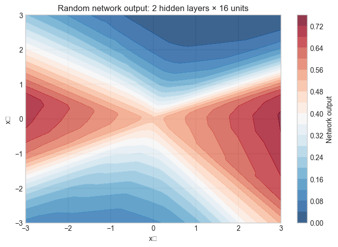
Architecture: [2, 16, 16, 1]
Total parameters: 337
# --- Experiment 2: What happens without nonlinearity? ---
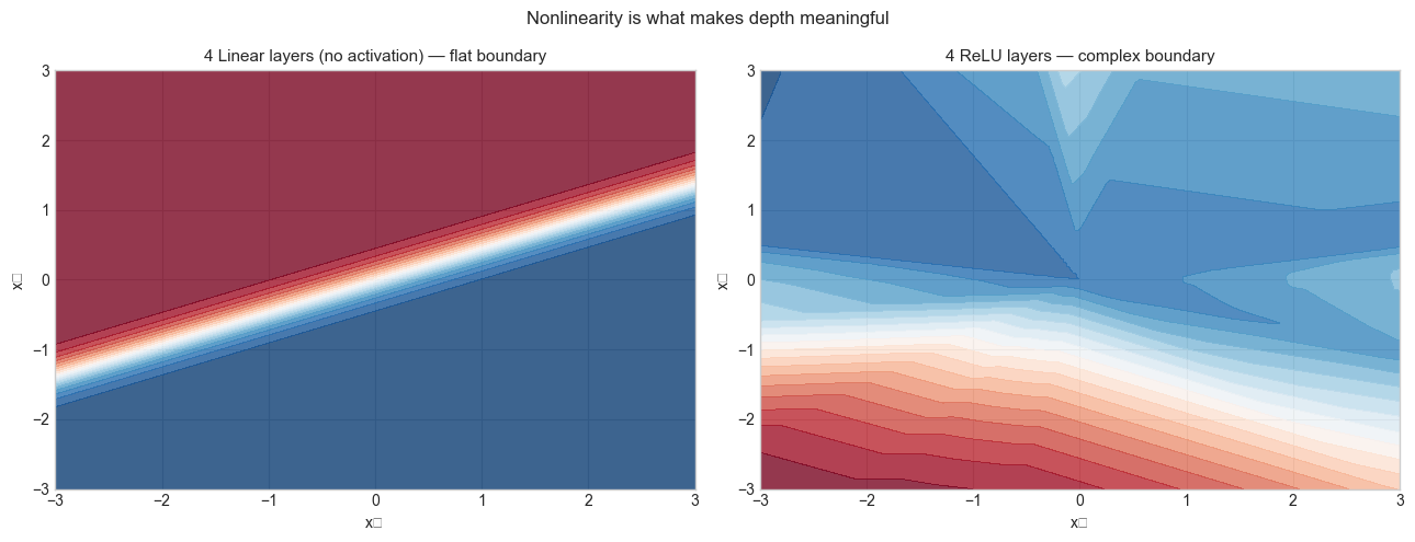
# Hypothesis: stacking linear layers without activation collapses to a single linear map
# Try changing: N_LAYERS to see that the boundary stays linear
def linear(z): return z # identity activation = no nonlinearity
N_LAYERS = 4 # <-- modify this
architecture_linear = [2] + [8] * N_LAYERS + [1]
net_linear = NeuralNetwork(architecture_linear, output_activation=sigmoid)
# Override hidden layer activations to identity
for layer in net_linear.layers[:-1]:
layer.activation = linear
preds_linear = net_linear.forward(grid).reshape(xx.shape)
fig, axes = plt.subplots(1, 2, figsize=(13, 5))
net_relu = NeuralNetwork([2] + [8] * N_LAYERS + [1])
preds_relu = net_relu.forward(grid).reshape(xx.shape)
axes[0].contourf(xx, yy, preds_linear, levels=20, cmap='RdBu_r', alpha=0.8)
axes[0].set_title(f'{N_LAYERS} Linear layers (no activation) — flat boundary', fontsize=11)
axes[0].set_xlabel('x₁'); axes[0].set_ylabel('x₂')
axes[1].contourf(xx, yy, preds_relu, levels=20, cmap='RdBu_r', alpha=0.8)
axes[1].set_title(f'{N_LAYERS} ReLU layers — complex boundary', fontsize=11)
axes[1].set_xlabel('x₁'); axes[1].set_ylabel('x₂')
plt.suptitle('Nonlinearity is what makes depth meaningful', fontsize=12)
plt.tight_layout(); plt.show()C:\Users\user\AppData\Local\Temp\ipykernel_2856\1589546560.py:30: UserWarning: Glyph 8321 (\N{SUBSCRIPT ONE}) missing from font(s) Arial.
plt.tight_layout(); plt.show()
C:\Users\user\AppData\Local\Temp\ipykernel_2856\1589546560.py:30: UserWarning: Glyph 8322 (\N{SUBSCRIPT TWO}) missing from font(s) Arial.
plt.tight_layout(); plt.show()
7. Exercises
Easy 1. A network has architecture [784, 256, 128, 10]. How many parameters (weights + biases) does it have in total? Compute by hand, then verify with code.
Easy 2. Why does x @ W.T + b give the same result as (W @ x.T).T + b when x is a batch? Verify with a small numeric example.
Medium 1. Modify DenseLayer to store the pre-activation values z as self.z and the post-activation values as self.h during the forward pass. These are needed for backpropagation. Verify that shapes are correct for both single and batch inputs.
Medium 2. Implement a tanh activation and compare the output distribution of a 3-layer network using ReLU vs tanh on the same random input. Which activation produces outputs closer to zero-centered? Why does this matter for training? (Hint: think about what zero-centered activations do to gradient magnitudes.)
Hard. Prove that a composition of linear layers (no nonlinearity) is equivalent to a single linear layer. Specifically: if each layer computes , show that for some matrix . What is in terms of the individual weight matrices? Verify numerically.
8. Mini Project
# --- Mini Project: Visualize how a 2-layer network partitions R² ---
# Problem: Given a trained (or random-initialized) 2-layer network,
#   visualize what each hidden neuron has learned to detect.
# Task: Plot the activation of each hidden neuron over the input grid.
#   This shows that each neuron is a half-space detector (for ReLU).

import numpy as np
import matplotlib.pyplot as plt
plt.style.use('seaborn-v0_8-whitegrid')

np.random.seed(7)
N_HIDDEN = 6   # <-- try 4, 8, 12

W1 = np.random.randn(N_HIDDEN, 2)
b1 = np.random.randn(N_HIDDEN)

# Input grid
xx, yy = np.meshgrid(np.linspace(-3, 3, 150), np.linspace(-3, 3, 150))
grid = np.c_[xx.ravel(), yy.ravel()]  # (22500, 2)

# Hidden activations: each column = one neuron's response
Z1 = grid @ W1.T + b1          # (22500, N_HIDDEN)
H1 = np.maximum(0, Z1)         # ReLU

# Plot each hidden neuron's activation
n_cols = 3
n_rows = int(np.ceil(N_HIDDEN / n_cols))
fig, axes = plt.subplots(n_rows, n_cols, figsize=(4 * n_cols, 3.5 * n_rows))
axes = axes.ravel()

for i in range(N_HIDDEN):
    act = H1[:, i].reshape(xx.shape)
    axes[i].contourf(xx, yy, act, levels=20, cmap='viridis')
    axes[i].set_title(f'Hidden neuron {i+1}', fontsize=10)
    axes[i].set_xlabel('x₁'); axes[i].set_ylabel('x₂')

for j in range(N_HIDDEN, len(axes)):
    axes[j].axis('off')

plt.suptitle('Each ReLU neuron activates on a half-space in R²', fontsize=13)
plt.tight_layout()
plt.show()

print("Each neuron computes: ReLU(w·x + b)")
print("The boundary between 0 and nonzero is the hyperplane w·x + b = 0")
print("A network combines these half-space detectors to carve out regions.")
9. Chapter Summary & Connections
A neural network forward pass is a composition of affine transformations (
W @ x + b) interleaved with elementwise nonlinearities.The weight matrix
Wis the linear transformation (ch164); it rotates, scales, and projects the input space.Without nonlinear activations, any depth of linear layers collapses to a single matrix multiplication — depth buys nothing.
Shape arithmetic (
n_out × n_in) governs every layer; getting shapes right is prerequisite to everything else.Batch processing vectorizes over multiple inputs simultaneously using matrix multiplication, exploiting hardware parallelism.
Backward connections:
This chapter applies ch154 (matrix multiplication), ch164 (linear transformations), and ch176 (matrix calculus) directly.
Forward connections:
ch178 — Linear Layers in Deep Learning: extends this to batched gradient computation and the full training loop.
ch216 — Backpropagation Intuition: the chain rule from ch176 will be applied to this exact forward pass to derive parameter gradients.
ch228 — Gradient-Based Learning: uses the network defined here as the model being optimized.
Going deeper: Deep Learning by Goodfellow, Bengio & Courville, Chapter 6 — covers the universal approximation theorem, which formalizes why depth + nonlinearity is sufficient to represent any continuous function.