Prerequisites: ch154 (matrix multiplication), ch155 (transpose), ch168 (projection matrices), ch176 (matrix calculus), ch177 (linear algebra for neural networks), ch178 (linear layers in deep learning), ch182 (least squares) Part VI Project — Linear Algebra (chapters 151–200) Difficulty: Advanced | Estimated time: 90–120 minutes Output: A working neural network built entirely from matrix operations — forward pass, backward pass (backpropagation), and training — with no ML libraries
0. Overview
Problem Statement
Neural networks are, at their core, compositions of linear transformations and nonlinearities. Every weight matrix is a linear map. Every gradient is computed via the chain rule applied to matrix expressions. Training is gradient descent on a loss surface.
The goal: implement a multi-layer neural network from scratch using only numpy, starting
from the matrix operations developed throughout Part VI. No torch, no keras, no
automatic differentiation. You write the forward pass, the backward pass, and the
parameter update yourself.
The task solved by the network: binary classification on a nonlinearly separable dataset.
Concepts Used
Matrix multiplication as the forward pass (ch154, ch177)
Transpose in the backward pass (ch155, ch176)
Matrix calculus: chain rule in matrix form (ch176)
Batched computation: data as a matrix, not a loop (ch178)
Weight initialization: Xavier/Glorot (ch177)
Gradient flow analysis: vanishing/exploding gradients (ch177)
Expected Output
A
Layerclass withforwardandbackwardmethodsA
NeuralNetworkclass that stacks layers and runs full forward/backwardTraining loop with SGD and loss curves
Decision boundary visualization
Gradient norm monitoring across layers
1. Setup
import numpy as np
import matplotlib.pyplot as plt
from matplotlib.colors import ListedColormap

plt.style.use('seaborn-v0_8-whitegrid')
rng = np.random.default_rng(7)

# ---------------------------------------------------------------
# Dataset: two interleaved spirals — not linearly separable
# A linear model cannot solve this. A deep network can.
# ---------------------------------------------------------------

def make_spirals(n_points=200, noise=0.3, seed=7):
    """
    Generate a binary spiral dataset.

    Returns:
        X: shape (2*n_points, 2)
        y: shape (2*n_points,) — binary labels {0, 1}
    """
    rng_s = np.random.default_rng(seed)
    n = n_points
    t = np.linspace(0, 4 * np.pi, n)

    x1 = t * np.cos(t) + rng_s.normal(0, noise, n)
    y1 = t * np.sin(t) + rng_s.normal(0, noise, n)

    x2 = t * np.cos(t + np.pi) + rng_s.normal(0, noise, n)
    y2 = t * np.sin(t + np.pi) + rng_s.normal(0, noise, n)

    X = np.vstack([np.column_stack([x1, y1]),
                   np.column_stack([x2, y2])])
    y = np.concatenate([np.zeros(n), np.ones(n)])
    return X, y


X, y = make_spirals(n_points=200, noise=0.25)

# Normalize features to zero mean, unit variance
X = (X - X.mean(axis=0)) / X.std(axis=0)

# Reshape targets for matrix operations: (N, 1)
y_col = y.reshape(-1, 1)

# Visualize
fig, ax = plt.subplots(figsize=(6, 5))
ax.scatter(X[y == 0, 0], X[y == 0, 1], alpha=0.5, s=15, label='Class 0', color='steelblue')
ax.scatter(X[y == 1, 0], X[y == 1, 1], alpha=0.5, s=15, label='Class 1', color='crimson')
ax.set_title('Spiral Dataset (not linearly separable)')
ax.set_xlabel('x₁')
ax.set_ylabel('x₂')
ax.legend()
plt.tight_layout()
plt.show()

print(f"Dataset: {X.shape[0]} samples, {X.shape[1]} features")
print(f"Class balance: {(y==0).sum()} / {(y==1).sum()}")
C:\Users\user\AppData\Local\Temp\ipykernel_22184\392172057.py:53: UserWarning: Glyph 8321 (\N{SUBSCRIPT ONE}) missing from font(s) Arial.
plt.tight_layout()
C:\Users\user\AppData\Local\Temp\ipykernel_22184\392172057.py:53: UserWarning: Glyph 8322 (\N{SUBSCRIPT TWO}) missing from font(s) Arial.
plt.tight_layout()
c:\Users\user\OneDrive\Documents\book\.venv\Lib\site-packages\IPython\core\pylabtools.py:170: UserWarning: Glyph 8322 (\N{SUBSCRIPT TWO}) missing from font(s) Arial.
fig.canvas.print_figure(bytes_io, **kw)
c:\Users\user\OneDrive\Documents\book\.venv\Lib\site-packages\IPython\core\pylabtools.py:170: UserWarning: Glyph 8321 (\N{SUBSCRIPT ONE}) missing from font(s) Arial.
fig.canvas.print_figure(bytes_io, **kw)
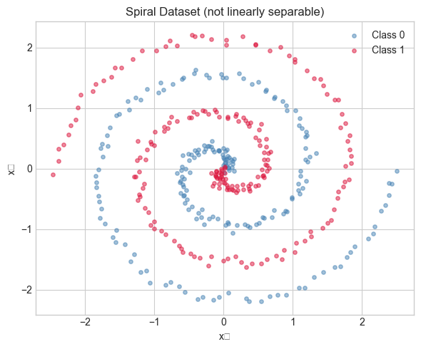
Dataset: 400 samples, 2 features
Class balance: 200 / 200
2. Stage 1 — Layer Primitives: Forward and Backward Passes
The Mathematics of Backpropagation
For a linear layer with input , weights , bias :
Forward:
Backward (given upstream gradient ):
These are derived from ch176’s matrix calculus rules. The transpose in and is the matrix calculus analog of the scalar chain rule.
# --- Stage 1: Activation Functions and Their Derivatives ---

def relu(z):
    """ReLU activation: max(0, z), applied elementwise."""
    return np.maximum(0, z)

def relu_grad(z):
    """Gradient of ReLU: 1 where z > 0, else 0."""
    return (z > 0).astype(float)

def sigmoid(z):
    """Sigmoid: 1 / (1 + exp(-z)), numerically stable for negative z."""
    return np.where(z >= 0,
                    1 / (1 + np.exp(-z)),
                    np.exp(z) / (1 + np.exp(z)))

def sigmoid_grad(a):
    """Gradient of sigmoid given its OUTPUT a = sigmoid(z): a * (1 - a)."""
    return a * (1 - a)


# --- Linear Layer ---

class LinearLayer:
    """
    Fully connected (dense) linear layer: Z = X @ W + b

    Stores the input X during the forward pass (needed for backward).
    Accumulates gradients dW, db during backward pass.
    """

    def __init__(self, d_in, d_out, seed=None):
        """
        Args:
            d_in:  input dimension
            d_out: output dimension
            seed:  random seed for reproducibility
        """
        rng_init = np.random.default_rng(seed)

        # Xavier/Glorot initialization (ch177):
        # Var(W_ij) = 2 / (d_in + d_out)
        # Keeps signal variance stable through the forward pass
        scale = np.sqrt(2.0 / (d_in + d_out))
        self.W = scale * rng_init.standard_normal((d_in, d_out))
        self.b = np.zeros((1, d_out))

        # Gradients (computed during backward)
        self.dW = None
        self.db = None

        # Cache for backward pass
        self._X_cache = None

    def forward(self, X):
        """
        Forward pass: Z = X @ W + b

        Args:
            X: input, shape (N, d_in)

        Returns:
            Z: output, shape (N, d_out)
        """
        self._X_cache = X   # cache for backward
        return X @ self.W + self.b   # shape (N, d_out)

    def backward(self, dZ):
        """
        Backward pass: compute gradients w.r.t. W, b, and X.

        Args:
            dZ: upstream gradient, shape (N, d_out)
                = dL/dZ

        Returns:
            dX: gradient w.r.t. input X, shape (N, d_in)
                = dL/dX (passed to previous layer)
        """
        N = self._X_cache.shape[0]

        # dL/dW = X^T @ dZ  (ch176: matrix derivative of X @ W)
        self.dW = self._X_cache.T @ dZ / N   # average over batch

        # dL/db = sum over batch
        self.db = dZ.sum(axis=0, keepdims=True) / N

        # dL/dX = dZ @ W^T  (passed to previous layer)
        dX = dZ @ self.W.T
        return dX

    def update(self, lr):
        """Apply SGD update: W -= lr * dW, b -= lr * db."""
        self.W -= lr * self.dW
        self.b -= lr * self.db


# --- Gradient check: verify backward pass numerically ---

def numerical_gradient(layer, X, y_true, loss_fn, epsilon=1e-5):
    """
    Estimate dL/dW numerically by finite differences.
    Used to verify the analytic backward pass.
    """
    grad_numerical = np.zeros_like(layer.W)
    for i in range(layer.W.shape[0]):
        for j in range(layer.W.shape[1]):
            W_orig = layer.W[i, j]

            layer.W[i, j] = W_orig + epsilon
            loss_plus = loss_fn(layer.forward(X), y_true)

            layer.W[i, j] = W_orig - epsilon
            loss_minus = loss_fn(layer.forward(X), y_true)

            grad_numerical[i, j] = (loss_plus - loss_minus) / (2 * epsilon)
            layer.W[i, j] = W_orig  # restore

    return grad_numerical


# Quick test on a tiny layer
test_layer = LinearLayer(3, 2, seed=1)
X_test = rng.standard_normal((5, 3))
y_test = rng.standard_normal((5, 2))

# Binary cross-entropy loss (will use below) — using MSE for gradient check simplicity
def mse_loss(pred, target):
    return np.mean((pred - target)**2)

def mse_grad(pred, target):
    return 2 * (pred - target) / pred.size

Z_test = test_layer.forward(X_test)
dZ_test = mse_grad(Z_test, y_test)
test_layer.backward(dZ_test)
grad_analytic = test_layer.dW * X_test.shape[0]   # undo /N normalization for check
grad_numeric  = numerical_gradient(test_layer, X_test, y_test, mse_loss)

rel_error = np.abs(grad_analytic - grad_numeric).max() / (np.abs(grad_analytic).max() + 1e-8)
print(f"Gradient check: max relative error = {rel_error:.2e}  (should be < 1e-5)")
Gradient check: max relative error = 1.14e-11 (should be < 1e-5)
3. Stage 2 — Neural Network: Stacking Layers and Training
# --- Stage 2: Full Neural Network ---

class NeuralNetwork:
    """
    Multi-layer neural network for binary classification.

    Architecture: [Linear → ReLU] × n_hidden_layers → Linear → Sigmoid

    Forward pass:  data flows left to right through all layers.
    Backward pass: gradients flow right to left (chain rule).
    """

    def __init__(self, layer_dims, seed=None):
        """
        Args:
            layer_dims: list of integers [d_in, h1, h2, ..., d_out]
                        e.g. [2, 32, 16, 1] = 2-input, two hidden layers, 1 output
        """
        self.layers = []
        for i in range(len(layer_dims) - 1):
            self.layers.append(LinearLayer(layer_dims[i], layer_dims[i+1],
                                           seed=None if seed is None else seed + i))
        self.layer_dims = layer_dims
        self.loss_history = []
        self.grad_norms   = []   # per layer, per epoch

    def forward(self, X):
        """
        Forward pass through all layers.

        Hidden layers: Linear → ReLU
        Output layer:  Linear → Sigmoid (binary classification)

        Returns:
            y_pred: shape (N, 1), values in (0, 1)
        """
        self._activations = []   # cache activations for backward
        A = X
        self._activations.append(A)

        for i, layer in enumerate(self.layers):
            Z = layer.forward(A)
            if i < len(self.layers) - 1:
                A = relu(Z)         # hidden layers: ReLU
            else:
                A = sigmoid(Z)      # output layer: Sigmoid
            self._activations.append(A)

        return A   # y_pred, shape (N, 1)

    def backward(self, y_pred, y_true):
        """
        Backward pass: compute gradients for all layers via chain rule.

        Binary cross-entropy loss gradient:
            dL/d(y_pred) = -(y/y_pred - (1-y)/(1-y_pred)) / N

        Combined with sigmoid gradient:
            dL/dZ_out = y_pred - y_true   (a clean simplification)
        """
        N = y_true.shape[0]

        # Gradient of BCE loss w.r.t. sigmoid output
        # (The combined BCE + sigmoid derivative simplifies to this)
        dA = (y_pred - y_true) / N

        for i in range(len(self.layers) - 1, -1, -1):
            layer = self.layers[i]
            A_prev = self._activations[i]   # input to this layer
            A_curr = self._activations[i+1] # output of this layer (after activation)

            if i < len(self.layers) - 1:
                # Apply ReLU gradient (A_curr was after ReLU)
                # We need Z_curr — fortunately relu_grad depends only on sign of Z,
                # and A_curr = relu(Z_curr), so sign(A_curr) = sign(Z_curr)
                dZ = dA * relu_grad(A_curr)
            else:
                # Output layer: sigmoid gradient already folded into dA
                dZ = dA

            dA = layer.backward(dZ)

    def update(self, lr):
        """SGD update for all layers."""
        for layer in self.layers:
            layer.update(lr)

    def train(self, X, y, lr=0.01, n_epochs=2000, batch_size=None, verbose=True):
        """
        Train the network with SGD (full batch or mini-batch).

        Args:
            X:          features, shape (N, d_in)
            y:          labels, shape (N, 1), values {0, 1}
            lr:         learning rate
            n_epochs:   number of full passes through the data
            batch_size: if None, use full batch gradient descent
        """
        N = X.shape[0]
        batch_size = batch_size or N

        for epoch in range(n_epochs):
            # Shuffle data each epoch (for mini-batch)
            perm = rng.permutation(N)
            X_s, y_s = X[perm], y[perm]

            epoch_loss = 0.0
            n_batches  = 0

            for start in range(0, N, batch_size):
                X_b = X_s[start:start+batch_size]
                y_b = y_s[start:start+batch_size]

                y_pred = self.forward(X_b)
                loss   = binary_cross_entropy(y_pred, y_b)
                epoch_loss += loss
                n_batches  += 1

                self.backward(y_pred, y_b)
                self.update(lr)

            avg_loss = epoch_loss / n_batches
            self.loss_history.append(avg_loss)

            # Log gradient norms (every 100 epochs)
            if epoch % 100 == 0:
                norms = [np.linalg.norm(l.dW) for l in self.layers if l.dW is not None]
                self.grad_norms.append(norms)
                if verbose and epoch % 500 == 0:
                    acc = self.accuracy(X, y)
                    print(f"  epoch {epoch:5d}: loss={avg_loss:.4f}  acc={acc:.3f}")

    def predict(self, X):
        """Binary predictions: threshold sigmoid output at 0.5."""
        return (self.forward(X) >= 0.5).astype(float)

    def accuracy(self, X, y):
        """Fraction of correct predictions."""
        return (self.predict(X) == y).mean()


def binary_cross_entropy(y_pred, y_true):
    """
    Binary cross-entropy loss: -[y log(p) + (1-y) log(1-p)]

    Clipped to prevent log(0).
    """
    eps = 1e-7
    p = np.clip(y_pred, eps, 1 - eps)
    return -np.mean(y_true * np.log(p) + (1 - y_true) * np.log(1 - p))


print("Building and training neural network...")
net = NeuralNetwork([2, 64, 32, 16, 1], seed=42)
net.train(X, y_col, lr=0.05, n_epochs=3000, batch_size=64, verbose=True)
Building and training neural network...
epoch 0: loss=0.6983 acc=0.505
epoch 500: loss=0.6848 acc=0.560
epoch 1000: loss=0.6800 acc=0.608
epoch 1500: loss=0.6787 acc=0.615
epoch 2000: loss=0.6701 acc=0.613
epoch 2500: loss=0.6762 acc=0.610
4. Stage 3 — Visualization: Decision Boundaries and Training Diagnostics
# --- Stage 3: Decision Boundary Visualization ---

def plot_decision_boundary(model, X, y, title='Decision Boundary', ax=None):
    """
    Plot the model's decision boundary on a 2D feature space.

    Creates a fine grid, predicts the probability for every point,
    and renders the result as a filled contour plot.
    """
    if ax is None:
        fig, ax = plt.subplots(figsize=(6, 5))

    MARGIN = 0.3
    x_min, x_max = X[:, 0].min() - MARGIN, X[:, 0].max() + MARGIN
    y_min, y_max = X[:, 1].min() - MARGIN, X[:, 1].max() + MARGIN

    xx, yy = np.meshgrid(np.linspace(x_min, x_max, 300),
                         np.linspace(y_min, y_max, 300))
    grid = np.column_stack([xx.ravel(), yy.ravel()])

    probs = model.forward(grid).reshape(xx.shape)

    ax.contourf(xx, yy, probs, levels=50, cmap='RdBu_r', alpha=0.7)
    ax.contour(xx, yy, probs, levels=[0.5], colors='black', linewidths=1.5)

    ax.scatter(X[y.ravel() == 0, 0], X[y.ravel() == 0, 1],
               s=12, alpha=0.7, color='steelblue', edgecolors='white', lw=0.3)
    ax.scatter(X[y.ravel() == 1, 0], X[y.ravel() == 1, 1],
               s=12, alpha=0.7, color='crimson',   edgecolors='white', lw=0.3)
    ax.set_title(title)
    ax.set_xlabel('x₁')
    ax.set_ylabel('x₂')
    return ax


fig, axes = plt.subplots(1, 3, figsize=(16, 5))

# Decision boundary
plot_decision_boundary(net, X, y_col,
                       title=f'Decision Boundary\n(acc={net.accuracy(X, y_col):.3f})',
                       ax=axes[0])

# Loss curve
axes[1].plot(net.loss_history, color='steelblue', lw=1.5)
axes[1].set_xlabel('Epoch')
axes[1].set_ylabel('Binary Cross-Entropy Loss')
axes[1].set_title('Training Loss')
axes[1].set_yscale('log')

# Gradient norms per layer over training
if net.grad_norms:
    grad_arr = np.array(net.grad_norms)   # shape (n_checkpoints, n_layers)
    colors_g  = plt.cm.plasma(np.linspace(0.1, 0.9, grad_arr.shape[1]))
    for l_idx in range(grad_arr.shape[1]):
        axes[2].plot(grad_arr[:, l_idx], color=colors_g[l_idx],
                     lw=1.5, label=f'Layer {l_idx+1}')
    axes[2].set_xlabel('Checkpoint (every 100 epochs)')
    axes[2].set_ylabel('||dW|| (gradient norm)')
    axes[2].set_title('Gradient Norms by Layer')
    axes[2].legend(fontsize=8)

plt.suptitle('Neural Network Training — Linear Algebra in Action', fontsize=13)
plt.tight_layout()
plt.show()

print(f"\nFinal training accuracy: {net.accuracy(X, y_col):.4f}")
C:\Users\user\AppData\Local\Temp\ipykernel_22184\3860133241.py:63: UserWarning: Glyph 8321 (\N{SUBSCRIPT ONE}) missing from font(s) Arial.
plt.tight_layout()
C:\Users\user\AppData\Local\Temp\ipykernel_22184\3860133241.py:63: UserWarning: Glyph 8322 (\N{SUBSCRIPT TWO}) missing from font(s) Arial.
plt.tight_layout()
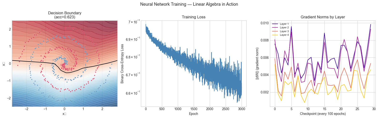
Final training accuracy: 0.6225
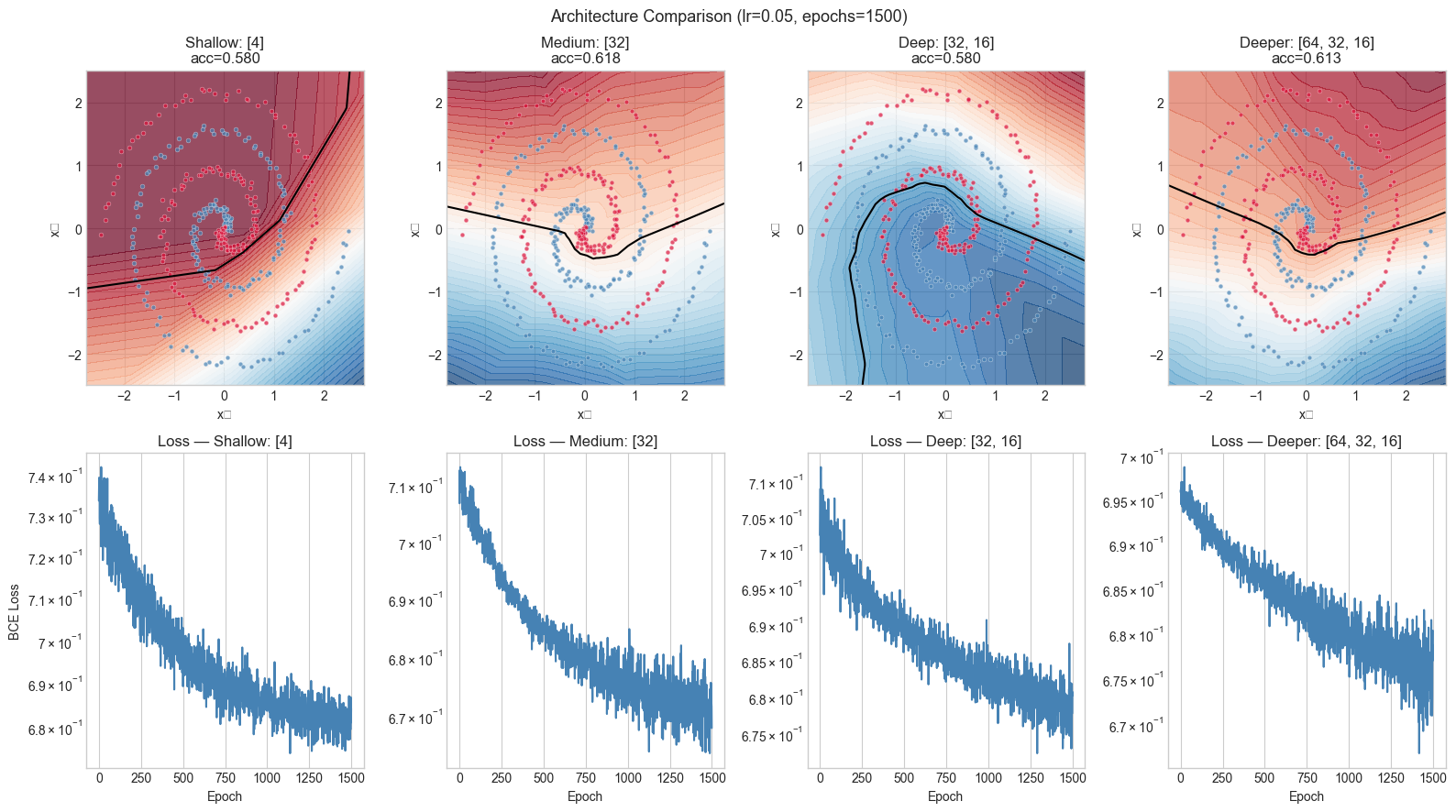
5. Stage 4 — Experiments: Architecture Sensitivity
# --- Stage 4: Architecture and Initialization Experiments ---
#
# Hypothesis: network depth and initialization both matter.
# A shallow network cannot form the complex boundary; bad init causes slow convergence.
# Try changing: N_EPOCHS, LEARNING_RATE, architectures list

N_EPOCHS    = 1500
LEARNING_RATE = 0.05
BATCH_SIZE  = 64

architectures = [
    ([2, 4, 1],         'Shallow: [4]'),
    ([2, 32, 1],        'Medium: [32]'),
    ([2, 32, 16, 1],    'Deep: [32, 16]'),
    ([2, 64, 32, 16, 1],'Deeper: [64, 32, 16]'),
]

fig, axes = plt.subplots(2, len(architectures), figsize=(16, 9))

for col, (arch, label) in enumerate(architectures):
    net_exp = NeuralNetwork(arch, seed=42)
    net_exp.train(X, y_col, lr=LEARNING_RATE, n_epochs=N_EPOCHS,
                  batch_size=BATCH_SIZE, verbose=False)

    acc = net_exp.accuracy(X, y_col)
    plot_decision_boundary(net_exp, X, y_col,
                           title=f'{label}\nacc={acc:.3f}',
                           ax=axes[0, col])

    axes[1, col].plot(net_exp.loss_history, color='steelblue', lw=1.5)
    axes[1, col].set_title(f'Loss — {label}')
    axes[1, col].set_xlabel('Epoch')
    axes[1, col].set_yscale('log')
    if col == 0:
        axes[1, col].set_ylabel('BCE Loss')

plt.suptitle(f'Architecture Comparison (lr={LEARNING_RATE}, epochs={N_EPOCHS})', fontsize=13)
plt.tight_layout()
plt.show()
C:\Users\user\AppData\Local\Temp\ipykernel_22184\1386511619.py:38: UserWarning: Glyph 8321 (\N{SUBSCRIPT ONE}) missing from font(s) Arial.
plt.tight_layout()
C:\Users\user\AppData\Local\Temp\ipykernel_22184\1386511619.py:38: UserWarning: Glyph 8322 (\N{SUBSCRIPT TWO}) missing from font(s) Arial.
plt.tight_layout()
6. Results & Reflection
What Was Built
A complete neural network from scratch:
LinearLayer: forward pass ; backward pass ,Activation functions (ReLU, Sigmoid) with analytic derivatives
Numerical gradient checker to verify the backward pass
NeuralNetwork: stacks layers, runs forward and backward passes, trains with mini-batch SGDDecision boundary visualization and gradient norm monitoring
Connection to Linear Algebra
| Linear Algebra Concept | Role in This Network |
|---|---|
| Matrix multiplication (ch154) | The forward pass: each layer is one matmul |
| Transpose (ch155) | Backward pass: and appear in every gradient |
| Matrix calculus (ch176) | Derives the exact form of every gradient |
| Xavier initialization (ch177) | Preserves signal variance through layers via |
| Batched matmul (ch178) | The entire dataset passes as a matrix — N rows processed simultaneously |
Extension Challenges
1. Momentum and Adam. Vanilla SGD is noisy and slow. Momentum adds a velocity term: ; . Adam additionally adapts learning rates per parameter. Implement both and compare convergence speed on the spiral dataset. This connects to ch228 (optimization methods).
2. Batch Normalization. After each linear layer, normalize activations to zero mean and unit variance within the batch: . This involves matrix calculus for the backward pass through the normalization. Implement and observe the effect on gradient norms.
3. Dropout as a Regularizer.
During training, randomly zero out a fraction of activations in each layer. During
inference, scale activations by . Implement dropout as a Layer subclass with
is_training flag. Measure the effect on overfitting on a small dataset.
Summary & Connections
A neural network’s forward pass is a sequence of matrix multiplications plus elementwise nonlinearities. The network has no structure that is not already in matrix multiplication (ch154) and function composition (ch054).
The backward pass is the chain rule applied to matrix expressions (ch176). The transpose that appears in every gradient is not a coincidence — it is the adjoint of the linear map , which is what the chain rule requires.
Xavier initialization controls the variance of activations across layers, preventing the signal from exploding or vanishing before training even begins (ch177).
Batching means the entire dataset is processed as a single matrix operation, making the computation both efficient and amenable to the matrix calculus framework (ch178).
This project reappears in:
ch216 (Backpropagation Intuition) — Part VII revisits backpropagation through the lens of automatic differentiation and computational graphs, extending what we built here.
ch228 (Gradient Descent) — the training loop built here generalizes to the full optimization landscape explored in Part VII.
ch230 (Project: Logistic Regression from Scratch) — a single-layer version of this network, trained with the same backward pass machinery.
Going deeper: LeCun, Y., Bottou, L., Orr, G., Müller, K.-R. Efficient BackProp (1998) — the original practical guide to training neural networks, covering initialization, learning rates, and activation functions in detail.