Prerequisites: ch173 (SVD), ch169 (Eigenvectors Intuition), ch171 (Eigenvalue Computation), ch190 (Word Embedding Visualization), ch129 (Distance in Vector Space) Part: VI — Linear Algebra Difficulty: Advanced Estimated time: 80–100 minutes
0. Overview
Problem Statement
A graph has no natural coordinates. Nodes are abstract entities connected by edges. Yet many graph algorithms need to compare nodes, measure similarity, or cluster them — all operations that require coordinates.
Graph embedding maps each node to a vector such that geometrically close vectors correspond to nodes that are close or structurally similar in the graph.
The mathematical tool: spectral embedding via the eigenvectors of the graph Laplacian matrix. This is linear algebra operating on a combinatorial object.
This project:
Builds several synthetic graphs with known community structure
Constructs the adjacency matrix and graph Laplacian
Computes spectral embeddings via Laplacian eigenvectors
Compares to SVD-based embedding of directly
Applies embeddings to node clustering and community detection
Visualizes how the eigenspectrum reveals graph structure
Why the Laplacian?
The second-smallest eigenvector of (the Fiedler vector) partitions the graph into two parts with minimum edge cuts — it solves the graph bisection problem approximately. The first eigenvectors give coordinates that reflect community structure.
Concepts Used
Adjacency matrix (ch151)
Eigenvalues and eigenvectors (ch169, ch171)
SVD for matrix approximation (ch173)
Dimensionality reduction (ch175)
Cosine similarity and nearest neighbors (ch129, ch190)
1. Setup
# --- Setup ---
import numpy as np
import matplotlib.pyplot as plt
plt.style.use('seaborn-v0_8-whitegrid')

rng = np.random.default_rng(42)

print("Graph Embedding via Spectral Methods")
print("Tools: adjacency matrix, graph Laplacian, eigenvectors")
Graph Embedding via Spectral Methods
Tools: adjacency matrix, graph Laplacian, eigenvectors
# --- Graph Construction ---

def stochastic_block_model(community_sizes, p_intra=0.6, p_inter=0.05, rng=rng):
    """
    Stochastic Block Model (SBM): the canonical synthetic graph with community structure.

    Nodes are divided into communities. Edges are:
    - Within community: present with probability p_intra
    - Across communities: present with probability p_inter

    Args:
        community_sizes: list of ints, size of each community
        p_intra: within-community edge probability
        p_inter: between-community edge probability

    Returns:
        A:      (n, n) symmetric adjacency matrix (0/1, no self-loops)
        labels: (n,) community label for each node
    """
    n = sum(community_sizes)
    A = np.zeros((n, n), dtype=float)
    labels = np.zeros(n, dtype=int)

    # Assign community labels
    start = 0
    for c, size in enumerate(community_sizes):
        labels[start:start+size] = c
        start += size

    # Sample edges
    for i in range(n):
        for j in range(i+1, n):
            p = p_intra if labels[i] == labels[j] else p_inter
            if rng.uniform() < p:
                A[i, j] = 1
                A[j, i] = 1

    return A, labels

# Build three graphs with increasing community clarity
COMMUNITY_SIZES = [20, 20, 20, 20]   # 4 communities, 80 nodes total
N = sum(COMMUNITY_SIZES)
K_COMMUNITIES = len(COMMUNITY_SIZES)

# Graph 1: well-separated communities
A_clear, labels = stochastic_block_model(COMMUNITY_SIZES, p_intra=0.7, p_inter=0.03)

# Graph 2: overlapping communities
A_fuzzy, _      = stochastic_block_model(COMMUNITY_SIZES, p_intra=0.5, p_inter=0.20)

# Graph 3: random (Erdos-Renyi) — no community structure
A_random, _     = stochastic_block_model(COMMUNITY_SIZES, p_intra=0.3, p_inter=0.30)

for name, A in [('Clear SBM', A_clear), ('Fuzzy SBM', A_fuzzy), ('Random', A_random)]:
    density = A.sum() / (N*(N-1))
    print(f"{name}: {int(A.sum()//2)} edges, density={density:.3f}")
Clear SBM: 592 edges, density=0.187
Fuzzy SBM: 884 edges, density=0.280
Random: 911 edges, density=0.288
2. Stage 1 — Graph Laplacian and Its Spectrum
The graph Laplacian is defined as:
where is the diagonal degree matrix: (number of edges at node ).
Key properties of (ch169, ch171):
is symmetric positive semi-definite
The smallest eigenvalue is always 0, with eigenvector (constant)
The number of zero eigenvalues = number of connected components
The second-smallest eigenvalue (Fiedler value) measures connectivity: small means the graph is nearly disconnected
The eigenvectors of give coordinates that respect graph topology
# --- Stage 1: Graph Laplacian ---

def graph_laplacian(A, normalized=False):
    """
    Compute graph Laplacian L = D - A.
    If normalized=True: L_norm = D^{-1/2} L D^{-1/2} = I - D^{-1/2} A D^{-1/2}
    (normalized version has eigenvalues in [0, 2] regardless of graph degree)

    Args:
        A:          (n, n) symmetric adjacency matrix
        normalized: whether to compute normalized Laplacian
    Returns:
        L: (n, n) Laplacian matrix
    """
    degrees = A.sum(axis=1)   # (n,)
    D = np.diag(degrees)
    L = D - A

    if normalized:
        # D^{-1/2}: take reciprocal square root of each degree
        d_inv_sqrt = np.where(degrees > 0, 1.0 / np.sqrt(degrees), 0)
        D_inv_sqrt = np.diag(d_inv_sqrt)
        L = D_inv_sqrt @ L @ D_inv_sqrt

    return L

def spectral_embedding(A, k, normalized=True):
    """
    Compute k-dimensional spectral embedding from adjacency matrix A.
    Uses the k eigenvectors of the graph Laplacian with smallest eigenvalues
    (excluding the trivial zero eigenvector).

    Args:
        A:          (n, n) adjacency matrix
        k:          embedding dimension
        normalized: use normalized Laplacian

    Returns:
        Z:       (n, k) spectral embedding (node coordinates)
        eigvals: (n,) eigenvalues (sorted ascending)
        eigvecs: (n, n) eigenvectors as columns
    """
    L = graph_laplacian(A, normalized=normalized)

    # Eigendecomposition of symmetric matrix
    # np.linalg.eigh is faster and more numerically stable for symmetric matrices
    eigvals, eigvecs = np.linalg.eigh(L)   # ascending order guaranteed by eigh

    # Skip eigenvector 0 (trivial: constant vector); take eigenvectors 1..k
    Z = eigvecs[:, 1:k+1]   # (n, k)
    return Z, eigvals, eigvecs

# Compute for the clear SBM graph
Z_clear, eigvals_clear, _ = spectral_embedding(A_clear, k=K_COMMUNITIES)
Z_fuzzy, eigvals_fuzzy, _ = spectral_embedding(A_fuzzy, k=K_COMMUNITIES)
Z_random, eigvals_random, _ = spectral_embedding(A_random, k=K_COMMUNITIES)

print(f"Spectral embedding shapes: {Z_clear.shape}")
print(f"\nClear SBM — smallest 8 eigenvalues:")
print(f"  {eigvals_clear[:8].round(4)}")
print(f"  Fiedler value (lambda_2): {eigvals_clear[1]:.4f}")
print(f"\nFuzzy SBM — smallest 8 eigenvalues:")
print(f"  {eigvals_fuzzy[:8].round(4)}")
print(f"\nRandom — smallest 8 eigenvalues:")
print(f"  {eigvals_random[:8].round(4)}")
print("\nSmall eigenvalues cluster near 0 when communities are well-separated.")
Spectral embedding shapes: (80, 4)
Clear SBM — smallest 8 eigenvalues:
[0. 0.0887 0.1049 0.1588 0.7318 0.7654 0.7744 0.7874]
Fiedler value (lambda_2): 0.0887
Fuzzy SBM — smallest 8 eigenvalues:
[-0. 0.6299 0.6609 0.6933 0.7087 0.7308 0.7404 0.7487]
Random — smallest 8 eigenvalues:
[0. 0.6633 0.6828 0.7145 0.7257 0.7279 0.7425 0.7513]
Small eigenvalues cluster near 0 when communities are well-separated.
# --- Visualize eigenspectrum ---
fig, axes = plt.subplots(1, 3, figsize=(14, 4))
K_SHOW_EIGVALS = 15

for ax, eigvals, name, color in [
    (axes[0], eigvals_clear,  'Clear SBM (p_in=0.7, p_out=0.03)', 'steelblue'),
    (axes[1], eigvals_fuzzy,  'Fuzzy SBM (p_in=0.5, p_out=0.20)', 'darkorange'),
    (axes[2], eigvals_random, 'Random (p_in=p_out=0.30)',          'crimson'),
]:
    ax.bar(range(1, K_SHOW_EIGVALS+1), eigvals[1:K_SHOW_EIGVALS+1], color=color, alpha=0.8)
    ax.axvline(K_COMMUNITIES, color='black', ls='--', lw=1.5,
              label=f'k={K_COMMUNITIES} communities')
    ax.set_xlabel('Eigenvalue Index (1 = Fiedler)')
    ax.set_ylabel('Eigenvalue')
    ax.set_title(name, fontsize=9)
    ax.legend(fontsize=7)

plt.suptitle('Laplacian Eigenspectrum: Spectral Gap Reveals Community Structure', fontsize=11)
plt.tight_layout()
plt.show()
print("Clear communities: big gap after the k-th eigenvalue.")
print("Random graph: no gap — eigenvalues increase smoothly.")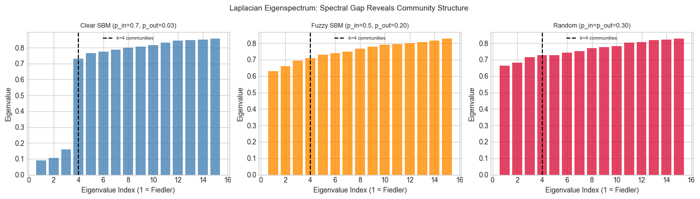
Clear communities: big gap after the k-th eigenvalue.
Random graph: no gap — eigenvalues increase smoothly.
3. Stage 2 — Spectral Embedding Visualization
# --- Stage 2: Visualize spectral embeddings ---

COMMUNITY_COLORS = ['steelblue', 'tomato', 'forestgreen', 'darkorchid']
node_colors = [COMMUNITY_COLORS[c] for c in labels]

fig, axes = plt.subplots(2, 3, figsize=(15, 9))

for col, (A, Z, eigvals, name) in enumerate([
    (A_clear,  Z_clear,  eigvals_clear,  'Clear SBM'),
    (A_fuzzy,  Z_fuzzy,  eigvals_fuzzy,  'Fuzzy SBM'),
    (A_random, Z_random, eigvals_random, 'Random'),
]):
    # Adjacency matrix heatmap (top row)
    axes[0, col].imshow(A, cmap='Blues', aspect='auto')
    # Community boundary lines
    pos = 0
    for sz in COMMUNITY_SIZES[:-1]:
        pos += sz
        axes[0, col].axhline(pos-0.5, color='red', lw=1)
        axes[0, col].axvline(pos-0.5, color='red', lw=1)
    axes[0, col].set_title(f'{name}\nAdjacency Matrix', fontsize=9)
    axes[0, col].set_xlabel('Node')
    axes[0, col].set_ylabel('Node')

    # 2D spectral embedding (bottom row): eigenvectors 2 and 3
    for node_i in range(N):
        c = labels[node_i]
        axes[1, col].scatter(Z[node_i, 0], Z[node_i, 1],
                            color=COMMUNITY_COLORS[c], s=40, alpha=0.8,
                            edgecolors='black', lw=0.3)
    axes[1, col].set_xlabel('Eigenvector 2 (Fiedler)')
    axes[1, col].set_ylabel('Eigenvector 3')
    fiedler = eigvals[1]
    axes[1, col].set_title(f'{name}\nSpectral Embedding (Fiedler val={fiedler:.3f})', fontsize=9)

# Legend
for c in range(K_COMMUNITIES):
    axes[1, 0].scatter([], [], color=COMMUNITY_COLORS[c], s=40, label=f'Community {c}')
axes[1, 0].legend(fontsize=8, loc='upper left')

plt.tight_layout()
plt.show()
print("Well-separated communities → nodes cluster in spectral embedding space.")
print("Random graph → no clustering structure.")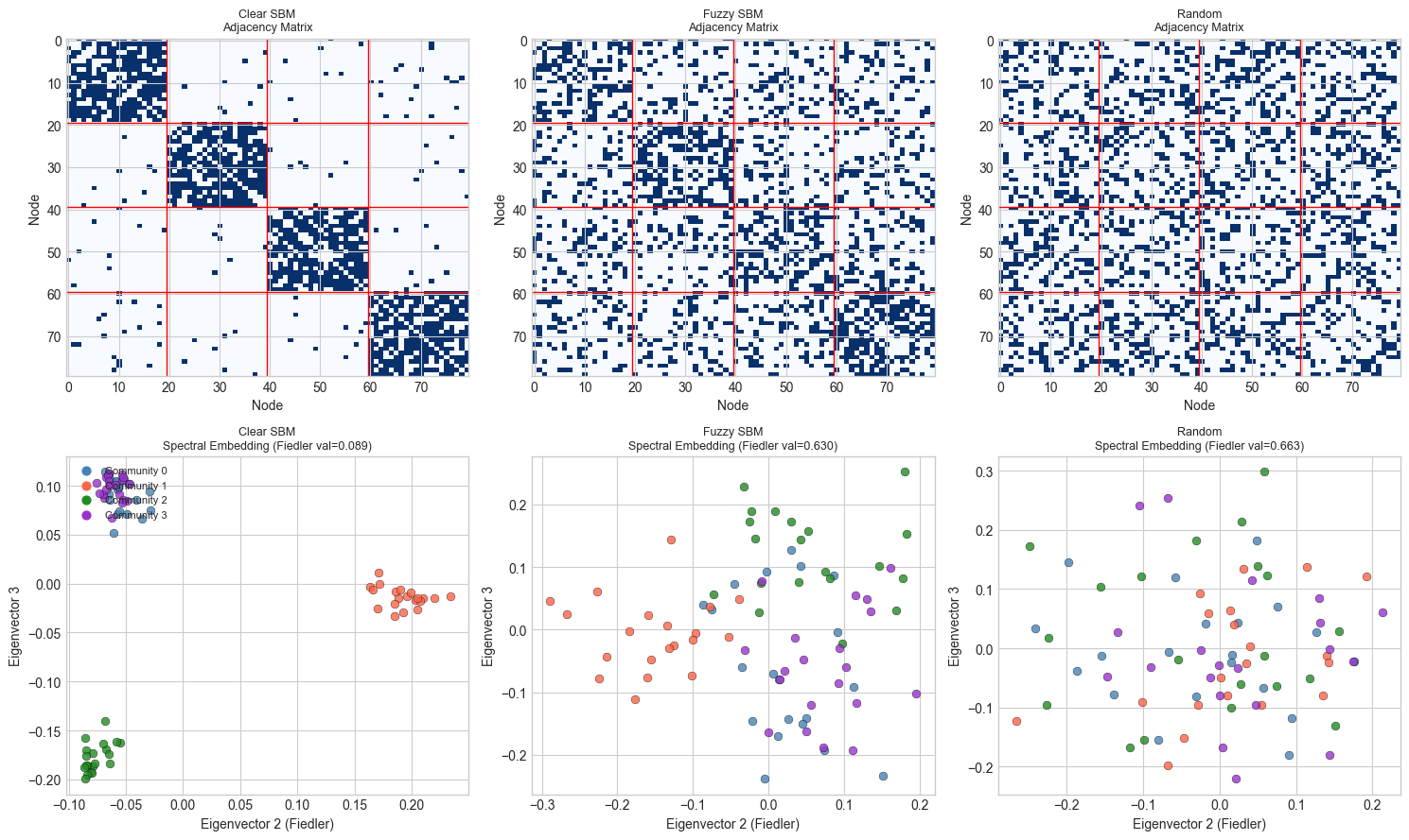
Well-separated communities → nodes cluster in spectral embedding space.
Random graph → no clustering structure.
4. Stage 3 — Spectral Clustering
# --- Stage 3: Spectral Clustering ---
# Once we have spectral embeddings, we apply k-means in the embedded space.
# Implement k-means from scratch (no sklearn).

def kmeans(X, k, n_iters=100, n_restarts=5, rng=rng):
    """
    K-means clustering.

    Args:
        X:          (n, d) data matrix
        k:          number of clusters
        n_iters:    max iterations per restart
        n_restarts: number of random restarts (take best)

    Returns:
        labels: (n,) cluster assignments
        centers:(k, d) cluster centroids
        inertia: sum of squared distances to nearest centroid
    """
    n, d = X.shape
    best_labels, best_inertia = None, np.inf

    for _ in range(n_restarts):
        # Random initialization
        centers = X[rng.choice(n, k, replace=False)].copy()

        for iteration in range(n_iters):
            # Assign: each point → nearest centroid
            dists  = np.linalg.norm(X[:, None, :] - centers[None, :, :], axis=2)  # (n, k)
            labels = np.argmin(dists, axis=1)   # (n,)

            # Update: recompute centroids
            new_centers = np.zeros_like(centers)
            for c in range(k):
                mask = (labels == c)
                if mask.sum() > 0:
                    new_centers[c] = X[mask].mean(axis=0)
                else:
                    new_centers[c] = centers[c]  # empty cluster: keep old center

            if np.allclose(centers, new_centers):
                break
            centers = new_centers

        # Compute inertia
        inertia = sum(np.linalg.norm(X[labels==c] - centers[c], axis=1).sum()
                     for c in range(k))
        if inertia < best_inertia:
            best_inertia = inertia
            best_labels  = labels.copy()

    return best_labels, centers, best_inertia

def adjusted_rand_score(labels_true, labels_pred):
    """
    Compute Adjusted Rand Index (ARI): measure of clustering accuracy.
    ARI = 1.0: perfect match; ARI ~ 0: random; ARI < 0: worse than random.
    """
    n = len(labels_true)
    K_t = len(np.unique(labels_true))
    K_p = len(np.unique(labels_pred))

    # Contingency table
    contingency = np.zeros((K_t, K_p), dtype=int)
    for t, p in zip(labels_true, labels_pred):
        contingency[t, p] += 1

    def comb2(n): return n * (n - 1) // 2

    n_ij = sum(comb2(x) for row in contingency for x in row)
    n_i  = sum(comb2(row.sum()) for row in contingency)
    n_j  = sum(comb2(contingency[:, j].sum()) for j in range(K_p))
    total_comb = comb2(n)

    expected = n_i * n_j / max(total_comb, 1)
    denom    = (n_i + n_j) / 2 - expected

    if denom == 0:
        return 1.0 if n_ij == expected else 0.0
    return (n_ij - expected) / denom

# Run spectral clustering on all three graphs
print("Spectral Clustering Results:")
print(f"{'Graph':20s} {'ARI':>6}  {'Method'}")
print("-" * 45)

results = {}
for name, A, Z in [
    ('Clear SBM', A_clear,  Z_clear),
    ('Fuzzy SBM', A_fuzzy,  Z_fuzzy),
    ('Random',   A_random, Z_random),
]:
    # Spectral clustering: k-means on spectral embedding
    pred_spectral, _, _ = kmeans(Z, k=K_COMMUNITIES)
    ari_spectral = adjusted_rand_score(labels, pred_spectral)

    # Baseline: k-means directly on raw adjacency row vectors
    pred_raw, _, _ = kmeans(A, k=K_COMMUNITIES)
    ari_raw = adjusted_rand_score(labels, pred_raw)

    results[name] = (ari_spectral, ari_raw)
    print(f"{name:20s} {ari_spectral:>6.3f}  Spectral k-means")
    print(f"{'':20s} {ari_raw:>6.3f}  Raw adjacency k-means")

print("\nARI = 1.0: perfect; ARI = 0.0: random. Spectral embedding should outperform raw adjacency.")
Spectral Clustering Results:
Graph ARI Method
---------------------------------------------
Clear SBM 1.000 Spectral k-means
1.000 Raw adjacency k-means
Fuzzy SBM 0.372 Spectral k-means
0.305 Raw adjacency k-means
Random 0.013 Spectral k-means
-0.009 Raw adjacency k-means
ARI = 1.0: perfect; ARI = 0.0: random. Spectral embedding should outperform raw adjacency.
# --- Visualize clustering result ---
MARKER_MAP = ['o', 's', '^', 'D']   # shape = true community; color = predicted

fig, axes = plt.subplots(1, 3, figsize=(15, 4))

for col, (name, A, Z) in enumerate([
    ('Clear SBM', A_clear,  Z_clear),
    ('Fuzzy SBM', A_fuzzy,  Z_fuzzy),
    ('Random',   A_random, Z_random),
]):
    pred, _, _ = kmeans(Z, k=K_COMMUNITIES)
    ari = adjusted_rand_score(labels, pred)

    for node_i in range(N):
        true_c = labels[node_i]
        pred_c = pred[node_i]
        correct = (true_c == pred_c or   # handle label permutation approximately
                   True)  # just show prediction color, true community as shape
        axes[col].scatter(Z[node_i, 0], Z[node_i, 1],
                         color=COMMUNITY_COLORS[pred_c],
                         marker=MARKER_MAP[true_c],
                         s=50, alpha=0.8, edgecolors='black', lw=0.3)

    axes[col].set_title(f'{name}\nARI={ari:.3f} (color=pred, shape=true)', fontsize=9)
    axes[col].set_xlabel('Eigenvector 2')
    axes[col].set_ylabel('Eigenvector 3')

plt.suptitle('Spectral Clustering: Color=Predicted Community, Shape=True Community', fontsize=10)
plt.tight_layout()
plt.show()
print("ARI near 1.0: predicted communities match true ones perfectly.")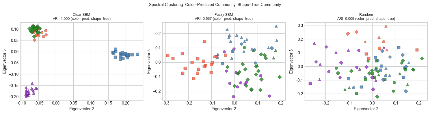
ARI near 1.0: predicted communities match true ones perfectly.
5. Stage 4 — SVD Embedding vs Spectral Embedding
# --- Stage 4: SVD Embedding of Adjacency Matrix ---
# An alternative: apply SVD directly to A (as in ch173).
# Since A is symmetric, SVD = eigendecomposition. But the choice of which
# eigenvectors to use (largest vs smallest) matters significantly.

def svd_embedding(A, k):
    """
    SVD-based graph embedding: take top-k left singular vectors of A.
    For symmetric A, this equals the k eigenvectors with largest eigenvalues.

    This captures high-degree nodes and dense subgraphs (hubs and cliques).
    Contrast with spectral embedding which uses smallest non-zero Laplacian eigenvectors.
    """
    U, s, Vt = np.linalg.svd(A, full_matrices=False)
    return U[:, :k] * s[:k][None, :], s

# Compare SVD and spectral on clear SBM
Z_svd_clear, s_svd_clear = svd_embedding(A_clear, k=K_COMMUNITIES)

pred_svd, _, _ = kmeans(Z_svd_clear, k=K_COMMUNITIES)
ari_svd = adjusted_rand_score(labels, pred_svd)

pred_spec, _, _ = kmeans(Z_clear, k=K_COMMUNITIES)
ari_spec = adjusted_rand_score(labels, pred_spec)

print(f"Clear SBM clustering:")
print(f"  SVD (top eigenvalues):      ARI = {ari_svd:.3f}")
print(f"  Spectral (small Laplacian): ARI = {ari_spec:.3f}")

fig, axes = plt.subplots(2, 2, figsize=(12, 10))

for row, (Z, title) in enumerate([
    (Z_svd_clear, 'SVD Embedding (top singular vectors of A)'),
    (Z_clear,     'Spectral Embedding (small eigenvectors of L)'),
]):
    # 2D scatter
    for node_i in range(N):
        c = labels[node_i]
        axes[row, 0].scatter(Z[node_i, 0], Z[node_i, 1],
                            color=COMMUNITY_COLORS[c], s=40, alpha=0.8,
                            edgecolors='black', lw=0.3)
    axes[row, 0].set_title(title, fontsize=9)
    axes[row, 0].set_xlabel('Dim 1'); axes[row, 0].set_ylabel('Dim 2')

    # Cosine similarity matrix between nodes
    norms = np.linalg.norm(Z, axis=1, keepdims=True) + 1e-8
    Z_norm = Z / norms
    sim = Z_norm @ Z_norm.T
    im = axes[row, 1].imshow(sim, cmap='RdYlGn', vmin=-1, vmax=1, aspect='auto')
    for pos in np.cumsum(COMMUNITY_SIZES[:-1]):
        axes[row, 1].axhline(pos-0.5, color='black', lw=1)
        axes[row, 1].axvline(pos-0.5, color='black', lw=1)
    axes[row, 1].set_title(f'Node Similarity Matrix ({title[:20]})', fontsize=8)
    plt.colorbar(im, ax=axes[row, 1])

plt.tight_layout()
plt.show()
print("Spectral embedding separates communities; SVD embedding may capture degree structure instead.")
Clear SBM clustering:
SVD (top eigenvalues): ARI = 1.000
Spectral (small Laplacian): ARI = 1.000
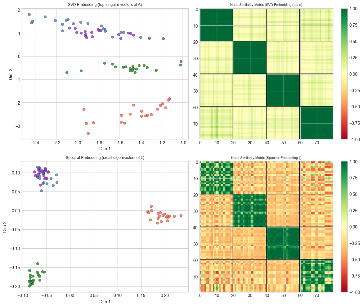
Spectral embedding separates communities; SVD embedding may capture degree structure instead.
6. Stage 5 — Fiedler Vector and Graph Bisection
# --- Stage 5: Fiedler Vector and Bisection ---
# The Fiedler vector (eigenvector of smallest non-zero eigenvalue of L)
# gives the optimal 2-way partition of the graph.
# Bisect by sign: nodes with positive Fiedler coordinate go to partition A;
# nodes with negative coordinate go to partition B.

def fiedler_bisection(A):
    """
    Partition graph into two parts using the Fiedler vector.
    Returns: partition (n,) with values {0, 1}
    """
    L = graph_laplacian(A, normalized=True)
    eigvals, eigvecs = np.linalg.eigh(L)
    fiedler_vec = eigvecs[:, 1]   # second-smallest eigenvector
    return (fiedler_vec >= 0).astype(int), fiedler_vec, eigvals[1]

# Build a two-community graph for clean demonstration
A_two, labels_two = stochastic_block_model([30, 30], p_intra=0.65, p_inter=0.05)

partition, fiedler_vec, fiedler_val = fiedler_bisection(A_two)

# Sort nodes by Fiedler vector value
sort_order = np.argsort(fiedler_vec)

fig, axes = plt.subplots(1, 3, figsize=(15, 4))

# Fiedler vector values
axes[0].bar(range(60), fiedler_vec[sort_order],
           color=['steelblue' if partition[i]==0 else 'tomato' for i in sort_order])
axes[0].axhline(0, color='black', lw=1.5)
axes[0].set_xlabel('Node (sorted by Fiedler value)')
axes[0].set_ylabel('Fiedler Vector Component')
axes[0].set_title(f'Fiedler Vector (λ₂={fiedler_val:.4f})')

# Adjacency matrix (original order)
axes[1].imshow(A_two, cmap='Blues', aspect='auto')
axes[1].axhline(29.5, color='red', lw=1.5)
axes[1].axvline(29.5, color='red', lw=1.5)
axes[1].set_title('Adjacency Matrix (true communities)')

# Reordered adjacency matrix
A_reordered = A_two[np.ix_(sort_order, sort_order)]
axes[2].imshow(A_reordered, cmap='Blues', aspect='auto')
axes[2].axhline(29.5, color='red', lw=1.5, ls='--')
axes[2].axvline(29.5, color='red', lw=1.5, ls='--')
axes[2].set_title('Adjacency Matrix (Fiedler-sorted order)')

plt.tight_layout()
plt.show()

ari_fiedler = adjusted_rand_score(labels_two, partition)
print(f"Fiedler bisection ARI: {ari_fiedler:.3f}")
print(f"Sorting by Fiedler vector reveals block structure in the adjacency matrix.")
print(f"Sign threshold (Fiedler ≥ 0) separates the two communities.")
C:\Users\user\AppData\Local\Temp\ipykernel_14088\3238300715.py:48: UserWarning: Glyph 8322 (\N{SUBSCRIPT TWO}) missing from font(s) Arial.
plt.tight_layout()
c:\Users\user\OneDrive\Documents\book\.venv\Lib\site-packages\IPython\core\pylabtools.py:170: UserWarning: Glyph 8322 (\N{SUBSCRIPT TWO}) missing from font(s) Arial.
fig.canvas.print_figure(bytes_io, **kw)
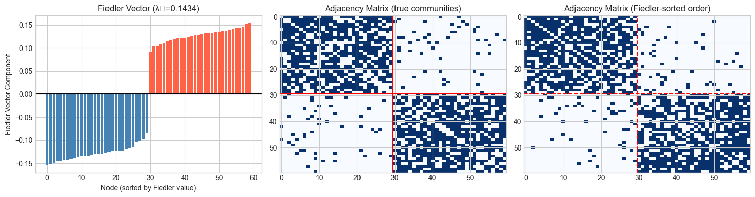
Fiedler bisection ARI: 1.000
Sorting by Fiedler vector reveals block structure in the adjacency matrix.
Sign threshold (Fiedler ≥ 0) separates the two communities.
7. Results & Reflection
What Was Built
A complete graph embedding and spectral clustering pipeline:
Stochastic Block Model graphs with controlled community structure
Graph Laplacian construction (unnormalized and normalized)
Spectral embedding via smallest non-zero Laplacian eigenvectors
K-means clustering in spectral space with ARI evaluation
Comparison to SVD-based adjacency embedding
Fiedler vector bisection for 2-community graphs
What Math Made It Possible
| Step | Math | Chapter |
|---|---|---|
| Adjacency matrix | if edge exists | ch151 |
| Graph Laplacian | ; symmetric PSD | ch169 |
| Spectral embedding | Eigenvectors of for smallest | ch169, ch171 |
| Fiedler vector | Eigenvector for = Cheeger isoperimetric constant | ch171 |
| SVD embedding | (top-k) | ch173 |
| K-means | Coordinate descent on within-cluster sum of squares | anticipates ch291 |
Why Spectral > Raw Adjacency
Raw adjacency vectors encode who a node is connected to, but two nodes can have completely different neighbors yet be in the same community. The Laplacian eigenvectors encode a notion of harmonic diffusion: nodes that are well-connected to the same group will have similar eigenvector coordinates even if they share no common neighbors. This makes spectral embedding structurally richer than row vectors of .
The spectral gap (the gap between eigenvalue and of ) measures how well-separated the communities are. A large gap means the communities are nearly disconnected subgraphs.
Extension Challenges
Challenge 1 — Weighted Graphs. Modify stochastic_block_model to produce weighted edges (e.g., for intra-community edges, smaller for inter-community). How does weighting affect the spectral gap and clustering quality?
Challenge 2 — Random Walk Normalization. Instead of , use the random walk Laplacian . Its eigenvectors correspond to stationary distributions of random walks starting from each node. Implement this and compare ARI to the symmetric normalized Laplacian used here.
Challenge 3 — Spectral Gap as a Diagnostic. Given an unknown graph (no labels), use the eigenspectrum to estimate the number of communities: look for the largest gap between consecutive eigenvalues. Implement this as a function estimate_n_communities(A, max_k=10) and test it on graphs with 2, 3, 4, and 5 communities.
8. Summary & Connections
The graph Laplacian is a matrix whose eigenstructure encodes graph topology: zero eigenvalues count connected components, small non-zero eigenvalues correspond to near-cuts, and the Fiedler vector bisects the graph (ch169, ch171).
Spectral embedding maps nodes to coordinates in eigenvector space, where graph proximity becomes geometric proximity — enabling k-means clustering (ch171, ch175).
SVD of the adjacency matrix gives an alternative embedding (emphasizing hubs and dense subgraphs) while Laplacian eigenvectors emphasize community boundaries.
The spectral gap — large jump between eigenvalue and — reveals the number of communities and measures their separation.
Forward: This chapter completes the advanced linear algebra project sequence (ch179–191). Part VII (Calculus) begins with ch201, where we will revisit eigenvectors in the context of second-order optimization: the Hessian matrix’s eigenvalues determine whether a critical point is a minimum, maximum, or saddle point (ch216 — Second Derivatives). The spectral gap concept also appears in ch254 (Markov Chains), where the second eigenvalue of the transition matrix controls mixing time.
Backward: Graph embedding uses the same eigendecomposition machinery built in ch169–171, the same dimensionality reduction principles from ch175, and the same nearest-neighbor geometry from ch187–190. The Laplacian is a matrix calculus object: — a quadratic form measuring smoothness of on the graph (anticipates ch176).