ch200 — Linear Algebra: Review and Synthesis

Prerequisites: All of Part VI (ch151–199) You will learn:
How every concept in Part VI connects to every other
The unified view: linear maps, their geometry, their computation, their applications
Which tools to reach for in which situations
The bridge from linear algebra to Part VII (Calculus) Environment: Python 3.x, numpy, matplotlib

1. The Map of Part VI¶

Part VI covered linear algebra in five conceptual layers:

Layer 1 — Representation (ch151–158): How matrices store linear maps. Matrix arithmetic, transpose, identity, inverse, determinant. The question: what is this object?

Layer 2 — Solution (ch159–163): Systems of equations. Gaussian elimination, LU decomposition. The question: given $A\mathbf{x} = \mathbf{b}$ , find $\mathbf{x}$ .

Layer 3 — Geometry (ch164–168): Linear transformations as geometric operations — rotation, scaling, projection. The question: what does this matrix do to space?

Layer 4 — Structure (ch169–179): Eigenvectors, SVD, PCA, matrix calculus. The question: what are the intrinsic directions and scales of this map?

Layer 5 — Applications (ch180–200): Image compression, recommendation systems, neural networks, graph analysis, sparse solvers. The question: how do these tools solve real problems?

The thread connecting all layers: SVD. Every major result in linear algebra has an SVD interpretation.

2. The SVD as the Unifying Tool¶

import numpy as np
import matplotlib.pyplot as plt
plt.style.use('seaborn-v0_8-whitegrid')
rng = np.random.default_rng(42)

# Demonstrate: every major linear algebra concept via SVD
A = rng.normal(0, 1, (6, 4))
U, s, Vt = np.linalg.svd(A, full_matrices=True)

tol = 1e-10
r = int(np.sum(s > tol))

print('A =', A.shape, '  rank =', r)
print()
print('SVD gives us everything:')
print(f'  Rank:         {r}  (nonzero singular values)')
print(f'  Nullity:      {A.shape[1] - r}  (zero singular values, ch192)')
print(f'  Col space:    U[:, :r]  shape={U[:,:r].shape}  (ch192)')
print(f'  Null space:   Vt[r:].T  shape={Vt[r:].T.shape}  (ch192)')
print(f'  Row space:    Vt[:r].T  shape={Vt[:r].T.shape}  (ch192)')
print(f'  Pseudoinverse: V @ S+ @ U.T  (ch193)')
print(f'  Condition number: {s[0]/s[-1]:.2f}  (ch194)')
print(f'  Spectral norm: {s[0]:.4f}  (ch194)')
print(f'  Frobenius norm: {np.linalg.norm(s):.4f}  (ch194)')
print(f'  Nuclear norm: {s.sum():.4f}  (ch194)')
print(f'  Low-rank approx: U[:,:k] S[:k] Vt[:k]  (ch173, ch180)')
print(f'  PCA directions: Vt rows  (ch174)')
print(f'  Eigenfaces: Vt rows  (ch187)')
print(f'  Word embeddings: U @ sqrt(S)  (ch190)')

A = (6, 4)   rank = 4

SVD gives us everything:
  Rank:         4  (nonzero singular values)
  Nullity:      0  (zero singular values, ch192)
  Col space:    U[:, :r]  shape=(6, 4)  (ch192)
  Null space:   Vt[r:].T  shape=(4, 0)  (ch192)
  Row space:    Vt[:r].T  shape=(4, 4)  (ch192)
  Pseudoinverse: V @ S+ @ U.T  (ch193)
  Condition number: 5.15  (ch194)
  Spectral norm: 3.0261  (ch194)
  Frobenius norm: 4.0528  (ch194)
  Nuclear norm: 7.2828  (ch194)
  Low-rank approx: U[:,:k] S[:k] Vt[:k]  (ch173, ch180)
  PCA directions: Vt rows  (ch174)
  Eigenfaces: Vt rows  (ch187)
  Word embeddings: U @ sqrt(S)  (ch190)

3. Decision Map: Which Tool for Which Problem?¶

# Visual decision map for Part VI tools
fig, ax = plt.subplots(figsize=(12, 8))
ax.set_xlim(0, 10); ax.set_ylim(0, 10)
ax.axis('off')
ax.set_title('Part VI — Linear Algebra Tool Selection Guide', fontsize=13, fontweight='bold')

# Boxes with tool descriptions
boxes = [
    (5, 9.2, 'Problem: Solve Ax = b', 'white', 'black', 14),
    (2, 7.5, 'Square, full rank A?\n→ LU (ch163) or direct solve', '#d4e8ff', 'black', 9),
    (7, 7.5, 'Overdetermined (m>n)?\n→ Pseudoinverse/QR (ch193)', '#d4ffd4', 'black', 9),
    (2, 5.8, 'Large sparse A?\n→ CG or iterative (ch196)', '#ffe4d4', 'black', 9),
    (7, 5.8, 'Underdetermined (m<n)?\n→ Min-norm via SVD (ch193)', '#ffd4f0', 'black', 9),
    (5, 4.0, 'Need structure of A?', 'white', 'black', 12),
    (1.5, 2.5, 'Compression/approx:\n→ Truncated SVD (ch173,180)', '#d4e8ff', 'black', 9),
    (4.0, 2.5, 'Clustering/embedding:\n→ PCA/Spectral (ch174,191)', '#d4ffd4', 'black', 9),
    (6.5, 2.5, 'Stability/dynamics:\n→ Eigenvalues (ch169,199)', '#ffe4d4', 'black', 9),
    (9.0, 2.5, 'Large scale:\n→ Randomized SVD (ch197)', '#ffd4f0', 'black', 9),
]

for x, y, text, fc, ec, fs in boxes:
    ax.text(x, y, text, ha='center', va='center', fontsize=fs,
           bbox=dict(boxstyle='round,pad=0.4', facecolor=fc, edgecolor='gray', lw=1.5))

# Arrows
arrows = [(5,8.9,2,7.9), (5,8.9,7,7.9), (5,8.9,2,6.2), (5,8.9,7,6.2),
          (5,3.7,1.5,2.9), (5,3.7,4.0,2.9), (5,3.7,6.5,2.9), (5,3.7,9.0,2.9)]
for x1,y1,x2,y2 in arrows:
    ax.annotate('', xy=(x2,y2), xytext=(x1,y1),
               arrowprops=dict(arrowstyle='->', color='gray', lw=1.5))

plt.tight_layout()
plt.show()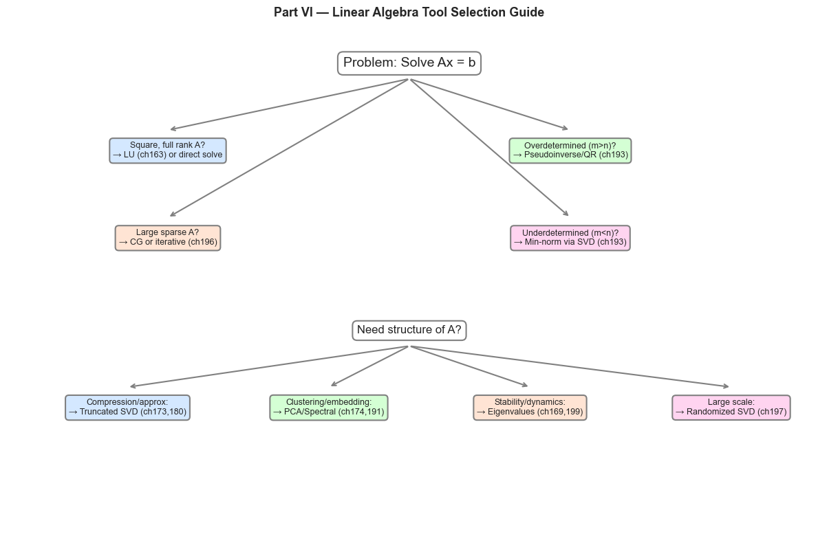

4. The Part VI → Part VII Bridge¶

Part VII (Calculus) starts where linear algebra ends. Here is how they connect:

Linear Algebra (Part VI)	Calculus (Part VII)
Matrix $A$ as a linear map	Jacobian $J(f)$ as the local linear approximation of $f$ (ch210)
Eigenvalues of $A$	Eigenvalues of the Hessian $H(f)$ determine saddle points (ch216)
SVD of $A$	SVD of the Jacobian in backpropagation (ch215)
Condition number $\kappa(A)$	Convergence rate of gradient descent on quadratic $\frac{1}{2}\mathbf{x}^\top A\mathbf{x}$ (ch212)
Null space of $A$	Directions of zero gradient (ch212)
Projection onto col $(A)$	Gradient projection in constrained optimization (ch218)
Matrix exponential $e^{At}$	Solution to linearized dynamics near equilibrium (ch225)
Conjugate Gradient (ch196)	Second-order optimizer for quadratic objectives (ch212)

The key insight: calculus replaces the matrix $A$ with the Jacobian or Hessian — a locally-valid linear approximation. All the tools from Part VI then apply to these local approximations.

5. Visualization¶

# Comprehensive demo: SVD applied to a real data-like matrix
# Shows rank, compression, PCA directions, and condition number in one view

# Synthetic structured data matrix (20 samples, 15 features, rank-3 structure)
n_samples, n_features, true_rank = 20, 15, 3
U_data = rng.normal(0,1,(n_samples, true_rank))
V_data = rng.normal(0,1,(n_features, true_rank))
X_data = U_data @ V_data.T + 0.3 * rng.normal(0,1,(n_samples, n_features))

U_svd, s_svd, Vt_svd = np.linalg.svd(X_data, full_matrices=False)

fig, axes = plt.subplots(2, 3, figsize=(14, 8))
fig.suptitle('SVD Analysis of a Structured Data Matrix', fontsize=12)

# Data matrix heatmap
im0 = axes[0,0].imshow(X_data, cmap='RdBu_r', aspect='auto')
axes[0,0].set_title('Data Matrix X (20×15)')
axes[0,0].set_xlabel('Feature'); axes[0,0].set_ylabel('Sample')
plt.colorbar(im0, ax=axes[0,0])

# Singular value spectrum
axes[0,1].bar(range(1, len(s_svd)+1), s_svd, color='steelblue', alpha=0.8)
axes[0,1].axvline(true_rank + 0.5, color='crimson', ls='--', label=f'True rank={true_rank}')
axes[0,1].set_xlabel('Index'); axes[0,1].set_ylabel('Singular value')
axes[0,1].set_title('Singular Value Spectrum')
axes[0,1].legend(fontsize=8)

# Low-rank reconstructions
errs = []
for k in range(1, 10):
    X_k = U_svd[:,:k] @ np.diag(s_svd[:k]) @ Vt_svd[:k]
    errs.append(np.linalg.norm(X_data - X_k, 'fro'))
axes[0,2].plot(range(1,10), errs, 'o-', ms=5, color='darkorange')
axes[0,2].axvline(true_rank, color='crimson', ls='--', label=f'True rank')
axes[0,2].set_xlabel('k'); axes[0,2].set_ylabel('Reconstruction error ||X-X_k||_F')
axes[0,2].set_title('Compression Quality vs Rank k')
axes[0,2].legend(fontsize=8)

# PCA 2D embedding (top-2 left singular vectors)
axes[1,0].scatter(U_svd[:,0]*s_svd[0], U_svd[:,1]*s_svd[1],
                  color='steelblue', s=60, edgecolors='black', lw=0.5)
axes[1,0].set_xlabel('PC 1'); axes[1,0].set_ylabel('PC 2')
axes[1,0].set_title('PCA Embedding (top-2 PCs)')

# Feature loadings
axes[1,1].scatter(Vt_svd[0], Vt_svd[1],
                  color='tomato', s=60, edgecolors='black', lw=0.5)
for j in range(n_features):
    axes[1,1].annotate(f'f{j}', (Vt_svd[0,j], Vt_svd[1,j]), fontsize=6)
axes[1,1].set_xlabel('PC 1 loading'); axes[1,1].set_ylabel('PC 2 loading')
axes[1,1].set_title('Feature Loadings')

# Condition number and norms summary
kappa = s_svd[0] / s_svd[-1]
axes[1,2].axis('off')
summary = [
    f'Shape:            {X_data.shape}',
    f'Rank (true):      {true_rank}',
    f'Rank (numerical): {int(np.sum(s_svd > 1e-10))}',
    f'Condition number: {kappa:.2f}',
    f'Spectral norm:    {s_svd[0]:.4f}',
    f'Frobenius norm:   {np.linalg.norm(X_data, "fro"):.4f}',
    f'Nuclear norm:     {s_svd.sum():.4f}',
    f'Variance in k=3:  {(s_svd[:3]**2).sum()/(s_svd**2).sum():.1%}',
]
for i, line in enumerate(summary):
    axes[1,2].text(0.05, 0.9 - i*0.11, line, transform=axes[1,2].transAxes,
                  fontsize=9, fontfamily='monospace')
axes[1,2].set_title('Matrix Properties Summary')

plt.tight_layout()
plt.show()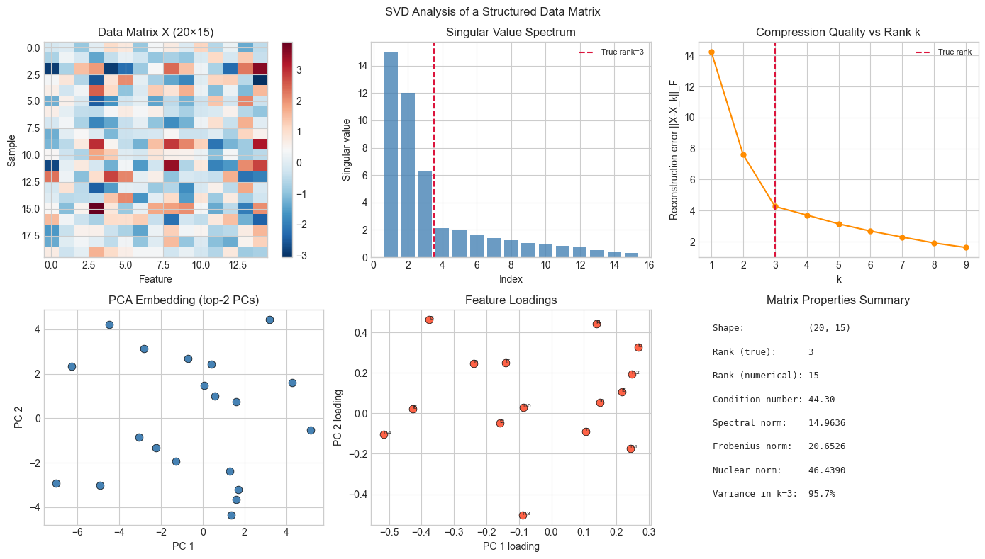

6. Mathematical Formulation¶

The central equation of Part VI is the SVD:

A = U \Sigma V^\top = \sum_{i=1}^r \sigma_i \mathbf{u}_i \mathbf{v}_i^\top

(1)

Every result in Part VI follows from understanding this decomposition:

Rank-Nullity (ch192): $r$ non-zero $\sigma_i$ ; null space spanned by remaining $\mathbf{v}_i$
Pseudoinverse (ch193): $A^+ = V\Sigma^+ U^\top$ , inverting only non-zero $\sigma_i$
Condition number (ch194): $\kappa = \sigma_1/\sigma_r$
Low-rank approximation (ch173, ch180): $A_k = \sum_{i=1}^k \sigma_i \mathbf{u}_i \mathbf{v}_i^\top$ minimizes Frobenius error
PCA (ch174): $\mathbf{v}_i$ are principal directions; $\sigma_i^2/(n-1)$ are explained variances
CG convergence (ch196, anticipates ch212): rate depends on $\kappa = \sigma_1/\sigma_r$
Randomized SVD (ch197): approximates $U_k, \Sigma_k, V_k$ in $O(mnk)$ time

7. Exercises — Synthesis¶

Easy 1. State the Rank-Nullity theorem and verify it for three matrices: $3\times5$ rank-2, $5\times3$ rank-3, and $4\times4$ rank-4. What does it mean geometrically?

Easy 2. For a $100\times20$ data matrix $X$ , describe step-by-step how you would: (a) find the top-3 principal components, (b) project all samples to 3D, (c) reconstruct approximate samples, (d) measure reconstruction error.

Medium 1. Build a pipeline that: generates a noisy low-rank matrix, computes randomized SVD (ch197), uses it to solve a least-squares problem (ch193), and evaluates stability of the resulting solution via condition number (ch194). Tie together at least 4 chapters.

Medium 2. The nuclear norm minimization problem: $\min_X \|X\|_* + \lambda\|A_\Omega(X) - b\|^2$ (where $A_\Omega$ observes only some entries) can be solved by iterative soft-thresholding of singular values. Implement one iteration and apply it to matrix completion (ch188 context).

Hard. The matrix completion problem (ch188, ch189) and the word embedding problem (ch190) both factor a matrix as $UV^\top$ with different loss structures. Show that both reduce to the same SVD problem when the observation pattern is complete, and explain why SVD is no longer optimal for sparse observations.

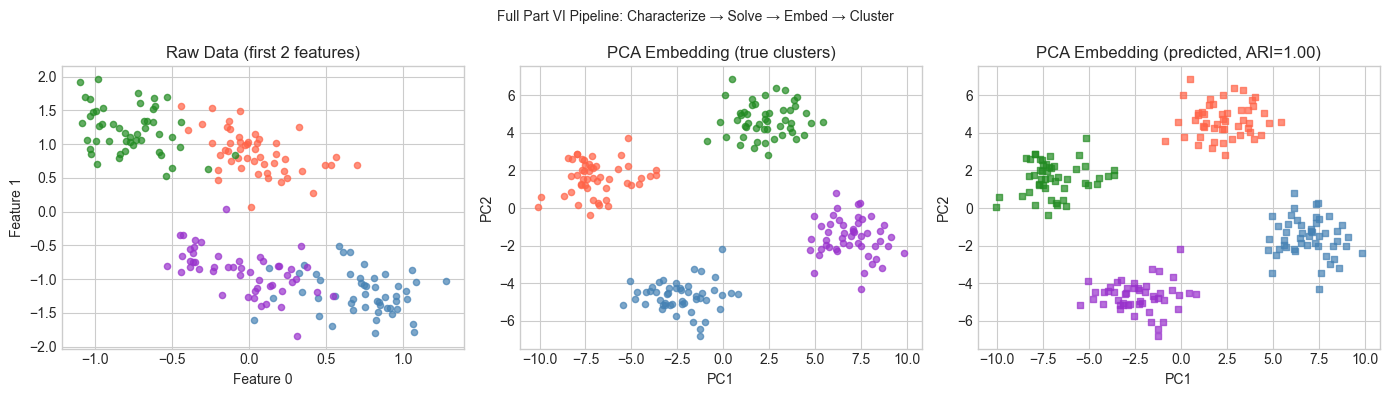
8. Mini Project¶

# --- Mini Project: Full Linear Algebra Pipeline ---
# Build a complete analysis pipeline that touches every layer of Part VI.
# Dataset: synthetic 2D point cloud from a mixture of Gaussians.

# Generate data
N_CLUSTERS = 4
N_PER     = 50
N_FEATURES = 20   # high-dimensional embedding

# Low-dimensional cluster centers
centers_2d = np.array([[2,2],[-2,2],[-2,-2],[2,-2]], dtype=float)

# Embed into high-D space via random linear map
embedding = rng.normal(0, 0.5, (2, N_FEATURES))  # 2D -> 20D
true_labels = []
X_hi = []
for c_i, center in enumerate(centers_2d):
    X_2d = center + rng.normal(0, 0.5, (N_PER, 2))
    X_hi.append(X_2d @ embedding + 0.2 * rng.normal(0, 1, (N_PER, N_FEATURES)))
    true_labels.extend([c_i] * N_PER)
X_data = np.vstack(X_hi)
true_labels = np.array(true_labels)

# --- Layer 1: Characterize the matrix ---
U_d, s_d, Vt_d = np.linalg.svd(X_data - X_data.mean(0), full_matrices=False)
kappa = s_d[0] / s_d[-1]
print(f'Shape: {X_data.shape}, Rank: {np.sum(s_d > 1e-10)}, κ={kappa:.2f}')

# --- Layer 2: Solve a least-squares problem ---
# Fit a linear model: predict feature 0 from features 1-19
A_ls = X_data[:, 1:]
b_ls = X_data[:, 0]
U_ls, s_ls, Vt_ls = np.linalg.svd(A_ls, full_matrices=False)
s_inv = np.where(s_ls > 1e-10, 1/s_ls, 0)
x_ls = Vt_ls.T @ (s_inv * (U_ls.T @ b_ls))
print(f'Least-squares residual: {np.linalg.norm(A_ls @ x_ls - b_ls):.4f}')

# --- Layer 3: PCA embedding ---
Z_2d = U_d[:, :2] * s_d[:2]  # top-2 PCA coordinates

# --- Layer 4: K-means in PCA space ---
def simple_kmeans(X, k, n_iters=50):
    centers = X[rng.choice(len(X), k, replace=False)]
    for _ in range(n_iters):
        dists  = np.linalg.norm(X[:,None,:] - centers[None,:,:], axis=2)
        labels = np.argmin(dists, axis=1)
        centers = np.array([X[labels==c].mean(0) if (labels==c).any() else centers[c]
                           for c in range(k)])
    return labels

pred_labels = simple_kmeans(Z_2d, N_CLUSTERS)

# ARI
def ari(t, p):
    k_t, k_p = len(np.unique(t)), len(np.unique(p))
    conf = np.zeros((k_t, k_p), dtype=int)
    for ti, pi in zip(t, p): conf[ti, pi] += 1
    c2 = lambda n: n*(n-1)//2
    n_ij = sum(c2(x) for row in conf for x in row)
    n_i  = sum(c2(row.sum()) for row in conf)
    n_j  = sum(c2(conf[:,j].sum()) for j in range(k_p))
    n    = len(t)
    exp  = n_i * n_j / max(c2(n), 1)
    denom = (n_i + n_j)/2 - exp
    return 0.0 if denom == 0 else (n_ij - exp) / denom

print(f'Clustering ARI: {ari(true_labels, pred_labels):.3f}  (1.0 = perfect)')

# --- Visualize ---
colors = ['steelblue','tomato','forestgreen','darkorchid']
fig, axes = plt.subplots(1, 3, figsize=(14, 4))

# Raw data (first 2 features)
for c in range(N_CLUSTERS):
    m = true_labels == c
    axes[0].scatter(X_data[m,0], X_data[m,1], color=colors[c], s=20, alpha=0.7)
axes[0].set_title('Raw Data (first 2 features)')
axes[0].set_xlabel('Feature 0'); axes[0].set_ylabel('Feature 1')

# PCA embedding (true labels)
for c in range(N_CLUSTERS):
    m = true_labels == c
    axes[1].scatter(Z_2d[m,0], Z_2d[m,1], color=colors[c], s=20, alpha=0.7)
axes[1].set_title('PCA Embedding (true clusters)')
axes[1].set_xlabel('PC1'); axes[1].set_ylabel('PC2')

# PCA embedding (predicted labels)
for c in range(N_CLUSTERS):
    m = pred_labels == c
    axes[2].scatter(Z_2d[m,0], Z_2d[m,1], color=colors[c], s=20, alpha=0.7, marker='s')
axes[2].set_title(f'PCA Embedding (predicted, ARI={ari(true_labels,pred_labels):.2f})')
axes[2].set_xlabel('PC1'); axes[2].set_ylabel('PC2')

plt.suptitle('Full Part VI Pipeline: Characterize → Solve → Embed → Cluster', fontsize=10)
plt.tight_layout()
plt.show()

Shape: (200, 20), Rank: 20, κ=36.53
Least-squares residual: 2.7065
Clustering ARI: 1.000  (1.0 = perfect)

9. Chapter Summary & Connections — The End of Part VI¶

What Part VI built:

A complete computational toolkit for linear transformations: representation (matrices), solution (elimination, SVD), geometric understanding (eigenvectors, projections), structure (low-rank decomposition), and application (compression, recommendation, embeddings, graphs).
The SVD as the single unifying tool: every major concept is a corollary of $A = U\Sigma V^\top$ .
Scale-awareness: direct methods for small systems, iterative methods (ch196) and randomized methods (ch197) for large ones.

What Part VII (Calculus) adds:

Non-linear functions replace matrices. The Jacobian $J(f)$ is the local matrix of $f$ at a point — and all of Part VI applies to it.
Derivatives become the primary object of study. ch204 (Derivatives) will revisit the matrix-vector product from a different angle: as the best linear approximation to a function near a point.
The Hessian is a matrix (symmetric, often positive definite) — its eigenvalues (ch169, ch171) determine whether a critical point is a minimum, maximum, or saddle (ch216).
Gradient descent is iterative solution of a linear system at the quadratic approximation — and its convergence rate depends on the condition number (ch194, ch196).

Forward: Part VII begins with ch201 (Why Calculus Matters) and builds through limits, derivatives, gradients, optimization, and backpropagation. Every chapter there will call back to Part VI.

Backward: Part VI built on Part V (Vectors, ch121–150) — vectors are the fundamental objects that matrices act on. Part VI’s dot product, norm, and projection geometry all originated there.