Part VII: Calculus
1. The Definition
The derivative of f at a point x is defined as the limit of the difference quotient:
This limit (introduced in ch203 — Limits Intuition) may or may not exist. When it exists, f is called differentiable at x.
The derivative is not a number — it is a function that tells you the instantaneous rate of change of f at every point where the limit exists.
The notation f’(x) is due to Leibniz’s alternative: df/dx. Both are standard. In this book we use f’(x) for clarity.
import numpy as np
import matplotlib.pyplot as plt

# Compute the derivative of f(x) = x^3 - x numerically and compare to analytical
f   = lambda x: x**3 - x
fp  = lambda x: 3*x**2 - 1  # analytical: d/dx (x^3 - x) = 3x^2 - 1

def numerical_derivative(f, x, h=1e-7):
    """Forward difference: [f(x+h) - f(x)] / h"""
    return (f(x + h) - f(x)) / h

x_vals = np.linspace(-2, 2, 400)

f_vals      = f(x_vals)
fp_exact    = fp(x_vals)
fp_numerical= numerical_derivative(f, x_vals)

fig, axes = plt.subplots(1, 2, figsize=(13, 5))

# Function and its derivative
axes[0].plot(x_vals, f_vals, color='steelblue', linewidth=2.5, label='f(x) = x³ - x')
axes[0].plot(x_vals, fp_exact, color='darkorange', linewidth=2, linestyle='--', label="f'(x) = 3x² - 1")
axes[0].axhline(0, color='gray', linewidth=0.8)
axes[0].set_title('f(x) and its derivative f\'(x)')
axes[0].legend()
axes[0].set_xlabel('x')

# Error between numerical and analytical
error = np.abs(fp_numerical - fp_exact)
axes[1].semilogy(x_vals, error + 1e-20, color='steelblue', linewidth=2)
axes[1].set_title('Error: |numerical - analytical|\n(should be ~1e-7 or less)')
axes[1].set_xlabel('x')
axes[1].set_ylabel('Absolute error')

plt.suptitle('Numerical vs Analytical Derivative', fontsize=13, fontweight='bold')
plt.tight_layout()
plt.show()

print(f'Max error across x ∈ [-2, 2]: {error.max():.2e}')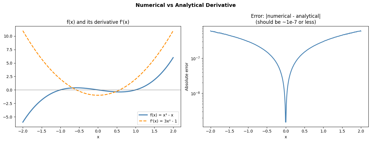
Max error across x ∈ [-2, 2]: 6.08e-07
2. Differentiation Rules
Rather than computing the limit every time, we use rules derived from the limit definition:
| Rule | Formula |
|---|---|
| Power rule | d/dx xⁿ = n·xⁿ⁻¹ |
| Constant | d/dx c = 0 |
| Sum | d/dx [f+g] = f’ + g’ |
| Product | d/dx [f·g] = f’g + fg’ |
| Chain rule | d/dx f(g(x)) = f’(g(x))·g’(x) |
| Exponential | d/dx eˣ = eˣ |
| Logarithm | d/dx ln(x) = 1/x |
| Sine / Cosine | d/dx sin(x) = cos(x), d/dx cos(x) = -sin(x) |
# Verify each rule numerically
h = 1e-7
numerical = lambda f, x: (f(x + h) - f(x)) / h

test_cases = [
    ('Power: x^4',        lambda x: x**4,          lambda x: 4*x**3,           np.array([1.5, -2.0, 0.5])),
    ('Exp: e^x',          lambda x: np.exp(x),      lambda x: np.exp(x),        np.array([0.0, 1.0, -1.0])),
    ('Log: ln(x)',        lambda x: np.log(x),      lambda x: 1/x,              np.array([0.5, 1.0, 3.0])),
    ('Sin: sin(x)',       lambda x: np.sin(x),      lambda x: np.cos(x),        np.array([0.0, np.pi/4, np.pi])),
    ('Product: x²·sin(x)',lambda x: x**2*np.sin(x), lambda x: 2*x*np.sin(x)+x**2*np.cos(x), np.array([1.0, 2.0])),
    ('Chain: sin(x²)',    lambda x: np.sin(x**2),   lambda x: 2*x*np.cos(x**2), np.array([1.0, 0.5])),
]

print(f'{"Rule":<25} {"x":>6}  {"Numerical":>14}  {"Analytical":>14}  {"Error":>10}')
print('-' * 78)

for name, f, fp_exact_fn, xs in test_cases:
    for x in xs:
        num = numerical(f, x)
        exact = fp_exact_fn(x)
        err = abs(num - exact)
        print(f'{name:<25} {x:>6.2f}  {num:>14.8f}  {exact:>14.8f}  {err:>10.2e}')
Rule x Numerical Analytical Error
------------------------------------------------------------------------------
Power: x^4 1.50 13.50000136 13.50000000 1.36e-06
Power: x^4 -2.00 -31.99999762 -32.00000000 2.38e-06
Power: x^4 0.50 0.50000015 0.50000000 1.50e-07
Exp: e^x 0.00 1.00000005 1.00000000 4.94e-08
Exp: e^x 1.00 2.71828197 2.71828183 1.40e-07
Exp: e^x -1.00 0.36787946 0.36787944 1.79e-08
Log: ln(x) 0.50 1.99999980 2.00000000 2.01e-07
Log: ln(x) 1.00 0.99999995 1.00000000 4.94e-08
Log: ln(x) 3.00 0.33333333 0.33333333 7.95e-09
Sin: sin(x) 0.00 1.00000000 1.00000000 1.67e-15
Sin: sin(x) 0.79 0.70710674 0.70710678 3.69e-08
Sin: sin(x) 3.14 -1.00000000 -1.00000000 1.64e-09
Product: x²·sin(x) 1.00 2.22324443 2.22324428 1.51e-07
Product: x²·sin(x) 2.00 1.97260210 1.97260236 2.62e-07
Chain: sin(x²) 1.00 1.08060450 1.08060461 1.14e-07
Chain: sin(x²) 0.50 0.96891251 0.96891242 8.38e-08
3. Where Derivatives Don’t Exist
Not every function is differentiable everywhere. Sharp corners, discontinuities, and vertical tangents are the common failure modes.
In machine learning, the ReLU activation function (introduced in ch065 — Activation Functions in ML) has a non-differentiable point at x=0. Practitioners use a subgradient (a generalization) at that point.
fig, axes = plt.subplots(1, 3, figsize=(14, 4))

# 1. |x| — not differentiable at 0 (corner)
x = np.linspace(-2, 2, 400)
axes[0].plot(x, np.abs(x), color='steelblue', linewidth=2, label='|x|')
# Left derivative = -1, right derivative = +1
axes[0].annotate('Corner — derivative\nnot defined here', xy=(0, 0), xytext=(0.5, 0.8),
                 arrowprops=dict(arrowstyle='->', color='red'), color='red', fontsize=9)
axes[0].set_title('|x|: corner at x=0')
axes[0].set_xlabel('x')

# 2. ReLU — derivative is 0 for x<0, 1 for x>0, undefined at 0
relu = lambda x: np.maximum(0, x)
drelu_subgrad = lambda x: np.where(x > 0, 1.0, 0.0)  # standard subgradient convention
axes[1].plot(x, relu(x), color='steelblue', linewidth=2, label='ReLU(x)')
axes[1].plot(x, drelu_subgrad(x), color='darkorange', linewidth=2, linestyle='--', label='subgradient')
axes[1].set_title('ReLU: corner at x=0\n(subgradient = 0 by convention)')
axes[1].set_xlabel('x')
axes[1].legend()

# 3. x^(1/3) — vertical tangent at 0
x3 = np.linspace(-2, 2, 400)
x3_nonzero = x3[x3 != 0]
cbrt = np.cbrt(x3)
dcbrt = np.where(x3 != 0, (1/3) * np.abs(x3)**(-2/3) * np.sign(x3), np.inf)
axes[2].plot(x3, cbrt, color='steelblue', linewidth=2, label='x^(1/3)')
axes[2].set_ylim(-2, 2)
axes[2].set_title('x^(1/3): vertical tangent at x=0\n(derivative → ∞)')
axes[2].set_xlabel('x')

plt.suptitle('Non-Differentiable Points', fontsize=13, fontweight='bold')
plt.tight_layout()
plt.show()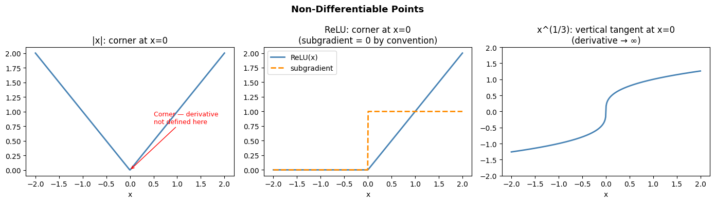
4. The Derivative as a Function
The derivative f’(x) is itself a function. We can ask about its properties:
Where is f’(x) = 0? (stationary points — potential minima/maxima)
Where is f’(x) > 0? (f is increasing)
Where is f’(x) < 0? (f is decreasing)
# f(x) = x^4 - 4x^2 (a double-well potential, common in physics and ML loss landscapes)
f   = lambda x: x**4 - 4*x**2
fp  = lambda x: 4*x**3 - 8*x

x = np.linspace(-2.5, 2.5, 500)

fig, axes = plt.subplots(1, 2, figsize=(13, 5))

# Annotate increasing/decreasing regions
axes[0].plot(x, f(x), color='steelblue', linewidth=2, label='f(x) = x⁴ - 4x²')
# Stationary points: f'(x) = 0 => 4x(x^2 - 2) = 0 => x = 0, ±√2
stationary = [0, np.sqrt(2), -np.sqrt(2)]
for xs in stationary:
    axes[0].scatter([xs], [f(xs)], color='red', zorder=6, s=80)
    axes[0].annotate(f'x={xs:.2f}\nf={f(xs):.2f}', xy=(xs, f(xs)),
                     xytext=(xs + 0.3, f(xs) + 1.5), fontsize=8)
axes[0].axhline(0, color='gray', linewidth=0.8)
axes[0].set_title('f(x) — double well\nRed dots: where f\'(x) = 0')
axes[0].legend()

axes[1].plot(x, fp(x), color='darkorange', linewidth=2, label="f'(x) = 4x³ - 8x")
axes[1].axhline(0, color='gray', linewidth=0.8)
axes[1].fill_between(x, fp(x), 0, where=fp(x) > 0, alpha=0.15, color='green', label="f'(x)>0 (increasing)")
axes[1].fill_between(x, fp(x), 0, where=fp(x) < 0, alpha=0.15, color='red', label="f'(x)<0 (decreasing)")
axes[1].set_title("f'(x) — derivative\nSign determines increase/decrease")
axes[1].legend(fontsize=9)

plt.suptitle('Reading the Derivative', fontsize=13, fontweight='bold')
plt.tight_layout()
plt.show()

print('Stationary points (where f\'(x) = 0):')
print(f'  x = 0    (local maximum): f(0) = {f(0)}')
print(f'  x = ±√2 (local minima):  f(±√2) = {f(np.sqrt(2)):.4f}')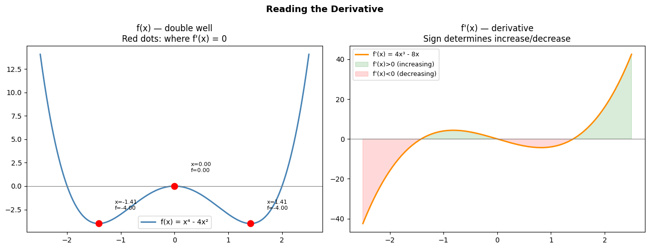
Stationary points (where f'(x) = 0):
  x = 0    (local maximum): f(0) = 0
  x = ±√2 (local minima):  f(±√2) = -4.0000
5. Summary
The derivative f’(x) = lim(h→0) [f(x+h)-f(x)]/h is the instantaneous rate of change
Differentiation rules (power, product, chain) are derived from this limit
Numerical derivatives approximate the limit with finite h; optimal h ≈ 1e-7
Derivatives can fail to exist at corners, discontinuities, and vertical tangents
Where f’(x) = 0: stationary points (potential optima); sign of f’(x) tells you increase/decrease
6. Forward References
The tangent line interpretation is developed geometrically in ch206 — Tangent Lines. The chain rule (listed in the table above) becomes central in ch215 — Chain Rule and ch216 — Backpropagation Intuition. The stationary point analysis above is extended to multiple dimensions in ch209 — Gradient Intuition and ch212 — Gradient Descent.