Part VII: Calculus
1. What a Partial Derivative Is
For a function of multiple variables f(x₁, x₂, ..., xₙ), the partial derivative with respect to xᵢ is the ordinary derivative of f treating all other variables as constants:
Notation: ∂f/∂xᵢ or fₓᵢ. The ∂ symbol (curly d) distinguishes partial from ordinary derivatives.
The gradient (ch209) is the vector of all partial derivatives: ∇f = [∂f/∂x₁, ..., ∂f/∂xₙ].
import numpy as np
import matplotlib.pyplot as plt

# f(x, y) = x^2 * sin(y)
# df/dx = 2x * sin(y)
# df/dy = x^2 * cos(y)

f    = lambda x, y: x**2 * np.sin(y)
dfdx = lambda x, y: 2*x * np.sin(y)
dfdy = lambda x, y: x**2 * np.cos(y)

# Numerical partial derivative via centered difference
h = 1e-7
num_dfdx = lambda x, y: (f(x+h, y) - f(x-h, y)) / (2*h)
num_dfdy = lambda x, y: (f(x, y+h) - f(x, y-h)) / (2*h)

# Verify at test points
test_points = [(1.0, 0.5), (2.0, np.pi/3), (-1.5, 1.0)]
print(f"{'Point':<20} {'df/dx (exact)':>14} {'df/dx (num)':>14} {'df/dy (exact)':>14} {'df/dy (num)':>14}")
print('-' * 80)
for x, y in test_points:
    ex_x = dfdx(x, y); nu_x = num_dfdx(x, y)
    ex_y = dfdy(x, y); nu_y = num_dfdy(x, y)
    print(f"({x:.1f}, {y:.2f})          {ex_x:>14.8f} {nu_x:>14.8f} {ex_y:>14.8f} {nu_y:>14.8f}")
Point                 df/dx (exact)    df/dx (num)  df/dy (exact)    df/dy (num)
--------------------------------------------------------------------------------
(1.0, 0.50)              0.95885108     0.95885108     0.87758256     0.87758256
(2.0, 1.05)              3.46410162     3.46410161     2.00000000     2.00000000
(-1.5, 1.00)             -2.52441295    -2.52441296     1.21568019     1.21568019
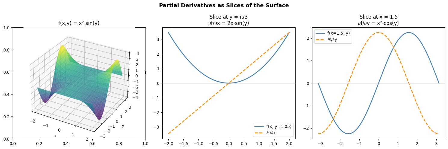
2. Visualizing Partial Derivatives
x_vals = np.linspace(-2, 2, 300)
y_fixed = np.pi / 3   # hold y constant

fig, axes = plt.subplots(1, 3, figsize=(15, 5))

# Surface
X, Y = np.meshgrid(np.linspace(-2, 2, 60), np.linspace(-np.pi, np.pi, 60))
Z = f(X, Y)
ax3d = fig.add_subplot(131, projection='3d')
ax3d.plot_surface(X, Y, Z, cmap='viridis', alpha=0.8)
ax3d.set_title('f(x,y) = x² sin(y)')
ax3d.set_xlabel('x'); ax3d.set_ylabel('y'); ax3d.set_zlabel('f')

# df/dx: slice at fixed y
axes[1].plot(x_vals, f(x_vals, y_fixed), color='steelblue', linewidth=2, label=f'f(x, y={y_fixed:.2f})')
axes[1].plot(x_vals, dfdx(x_vals, y_fixed), color='darkorange', linewidth=2, linestyle='--', label='∂f/∂x')
axes[1].axhline(0, color='gray', linewidth=0.8)
axes[1].set_title(f'Slice at y = π/3\n∂f/∂x = 2x·sin(y)')
axes[1].legend()

# df/dy: slice at fixed x
x_fixed = 1.5
y_vals = np.linspace(-np.pi, np.pi, 300)
axes[2].plot(y_vals, f(x_fixed, y_vals), color='steelblue', linewidth=2, label=f'f(x={x_fixed}, y)')
axes[2].plot(y_vals, dfdy(x_fixed, y_vals), color='darkorange', linewidth=2, linestyle='--', label='∂f/∂y')
axes[2].axhline(0, color='gray', linewidth=0.8)
axes[2].set_title(f'Slice at x = {x_fixed}\n∂f/∂y = x²·cos(y)')
axes[2].legend()

plt.suptitle('Partial Derivatives as Slices of the Surface', fontsize=13, fontweight='bold')
plt.tight_layout()
plt.show()
3. Partial Derivatives in the Loss Function
For a neural network with weight matrix W, the partial derivative ∂L/∂Wᵢⱼ tells us: how much does the loss change if we nudge weight Wᵢⱼ by a small amount? This is exactly what backpropagation computes (ch216).
# Partial derivatives of MSE for a linear model: L(w) = (1/N)||Xw - y||^2
# dL/dw_i = (2/N) * sum_j X_{ji} * (Xw - y)_j
# In matrix form: gradient = (2/N) * X^T (Xw - y)

np.random.seed(42)
N, D = 30, 3
X = np.random.randn(N, D)
w_true = np.array([1.5, -0.5, 2.0])
y = X @ w_true + 0.1 * np.random.randn(N)

w = np.array([0.0, 0.0, 0.0])

# Compute each partial derivative independently
h = 1e-7
partial_derivs = []
for i in range(D):
    w_plus  = w.copy(); w_plus[i]  += h
    w_minus = w.copy(); w_minus[i] -= h
    L_plus  = np.mean((X @ w_plus  - y)**2)
    L_minus = np.mean((X @ w_minus - y)**2)
    partial_derivs.append((L_plus - L_minus) / (2*h))

analytical_grad = (2/N) * X.T @ (X @ w - y)

print("Partial derivatives of MSE at w=0:")
print(f"{'Component':>12}  {'Numerical':>14}  {'Analytical':>14}  {'Error':>10}")
for i, (num, exact) in enumerate(zip(partial_derivs, analytical_grad)):
    print(f"dL/dw_{i}     {num:>14.8f}  {exact:>14.8f}  {abs(num-exact):>10.2e}")
Partial derivatives of MSE at w=0:
   Component       Numerical      Analytical       Error
dL/dw_0        -0.64083213     -0.64083213    2.66e-09
dL/dw_1         1.42689937      1.42689936    8.76e-09
dL/dw_2        -3.84072625     -3.84072626    1.27e-08
4. Summary
Partial derivative ∂f/∂xᵢ: derivative w.r.t. xᵢ, all other variables held constant
Computed with the same difference quotient as the ordinary derivative, applied to one variable
The gradient is the vector of all partial derivatives
Mixed partial derivatives: ∂²f/∂xᵢ∂xⱼ — the Hessian matrix collects these (ch217)
In ML: ∂L/∂wᵢⱼ for each weight is what gradient descent needs
5. Forward References
The collection of all partial derivatives of a vector-valued function — the Jacobian matrix — appears in ch215 — Chain Rule. The matrix of all second-order partial derivatives — the Hessian — is ch217 — Second Derivatives. Partial derivatives w.r.t. parameters in a neural network are computed by backpropagation in ch216.