Part VII: Calculus
1. The Algorithm
Gradient descent minimizes a function f(w) by iteratively stepping in the direction of the negative gradient:
where η (eta) is the learning rate — a hyperparameter controlling step size.
The negative gradient (ch209 — Gradient Intuition) points toward steepest decrease. Each step reduces f (for small enough η). Repeat until convergence.
This is not just an ML trick — it is a general optimization algorithm applicable to any differentiable scalar function.
import numpy as np
import matplotlib.pyplot as plt

def gradient_descent(f, grad_f, w0, lr, n_steps, tol=1e-9):
    """
    Run gradient descent from w0.
    Returns history of (w, f(w)) tuples.
    """
    w = np.array(w0, dtype=float)
    history = [(w.copy(), f(w))]
    for _ in range(n_steps):
        g = grad_f(w)
        w = w - lr * g
        history.append((w.copy(), f(w)))
        if np.linalg.norm(g) < tol:
            break
    return history

# Quadratic bowl: f(w1,w2) = w1^2 + 5*w2^2
f     = lambda w: w[0]**2 + 5*w[1]**2
grad_f = lambda w: np.array([2*w[0], 10*w[1]])

w0 = np.array([2.5, 1.5])
hist = gradient_descent(f, grad_f, w0, lr=0.08, n_steps=60)

path = np.array([h[0] for h in hist])
losses = [h[1] for h in hist]

# Contour + path
w1 = np.linspace(-3, 3, 200)
w2 = np.linspace(-2, 2, 200)
W1, W2 = np.meshgrid(w1, w2)
Z = W1**2 + 5*W2**2

fig, axes = plt.subplots(1, 2, figsize=(14, 5))

cs = axes[0].contourf(W1, W2, Z, levels=25, cmap='Blues', alpha=0.8)
axes[0].contour(W1, W2, Z, levels=10, colors='white', alpha=0.4, linewidths=0.8)
axes[0].plot(path[:, 0], path[:, 1], 'o-', color='red', markersize=4, linewidth=1.5, label='GD path')
axes[0].scatter(*w0, color='orange', s=100, zorder=8, label='start')
axes[0].scatter(0, 0, color='green', s=100, zorder=8, label='minimum')
axes[0].set_title(f'Gradient descent on f(w) = w₁² + 5w₂²\nLR={0.08}, {len(hist)-1} steps')
axes[0].legend(); axes[0].set_aspect('equal')

axes[1].semilogy(losses, color='steelblue', linewidth=2)
axes[1].set_xlabel('Step'); axes[1].set_ylabel('Loss (log scale)')
axes[1].set_title('Loss convergence')

plt.tight_layout()
plt.show()

print(f'Initial loss: {losses[0]:.4f}')
print(f'Final loss:   {losses[-1]:.2e}')
print(f'Converged to: {path[-1]}')
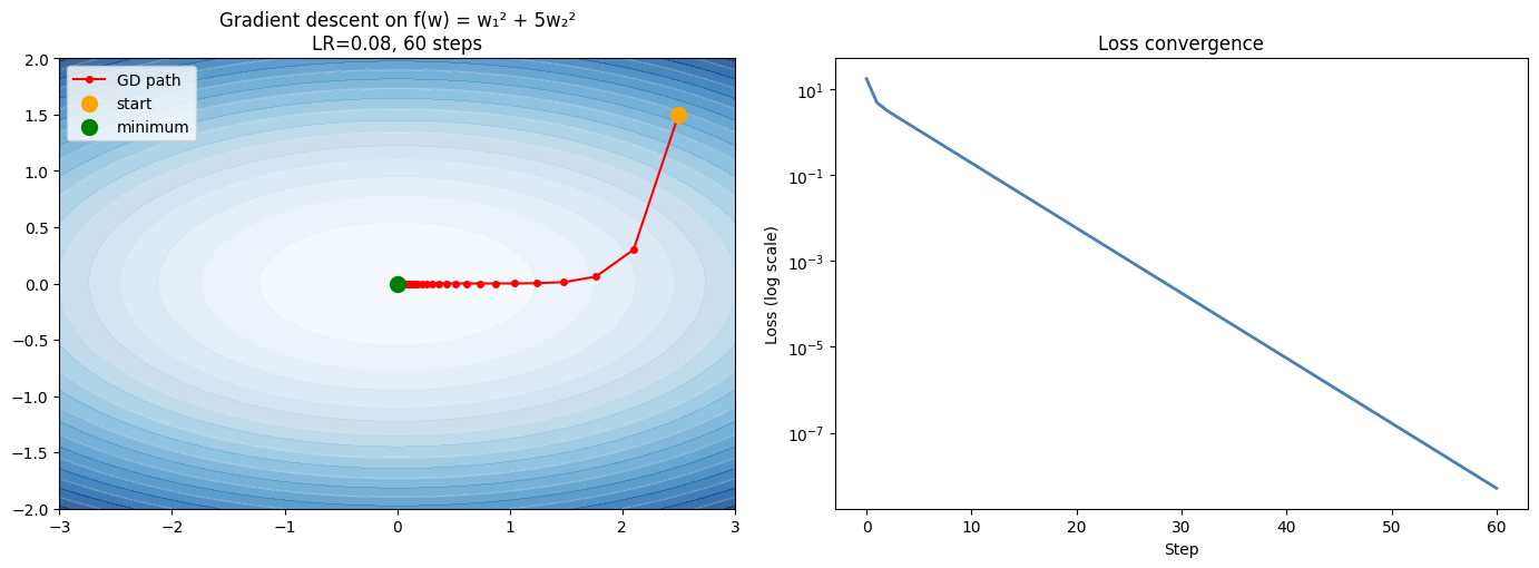
Initial loss: 17.5000
Final loss:   5.12e-09
Converged to: [7.15644227e-05 1.72938226e-42]
2. Learning Rate Effects
w0 = np.array([2.5, 1.5])
lrs = [0.01, 0.08, 0.15, 0.21]
colors = ['#3498db', '#2ecc71', '#e67e22', '#e74c3c']

fig, axes = plt.subplots(1, 2, figsize=(14, 5))

for lr, color in zip(lrs, colors):
    try:
        hist = gradient_descent(f, grad_f, w0, lr=lr, n_steps=100)
        losses = [h[1] for h in hist]
        path = np.array([h[0] for h in hist])
        axes[0].plot(losses[:50], color=color, linewidth=2, label=f'lr={lr}')
        axes[1].plot(path[:30, 0], path[:30, 1], 'o-', color=color,
                     markersize=3, linewidth=1.5, label=f'lr={lr}')
    except Exception as e:
        print(f'lr={lr} diverged: {e}')

axes[0].semilogy()
axes[0].set_xlabel('Step'); axes[0].set_ylabel('Loss')
axes[0].set_title('Effect of learning rate on convergence')
axes[0].legend()

cs = axes[1].contourf(W1, W2, Z, levels=20, cmap='Blues', alpha=0.6)
axes[1].contour(W1, W2, Z, levels=8, colors='white', alpha=0.3, linewidths=0.8)
axes[1].scatter(*w0, color='black', s=100, zorder=9, label='start')
axes[1].scatter(0, 0, color='green', s=100, zorder=9, label='minimum')
axes[1].set_title('Paths for different learning rates')
axes[1].legend(fontsize=8); axes[1].set_aspect('equal')

plt.tight_layout()
plt.show()

print('Observations:')
print('  Too small lr → slow convergence')
print('  Too large lr → oscillation or divergence')
print('  Optimal lr depends on curvature of the loss surface (Hessian eigenvalues, ch217)')
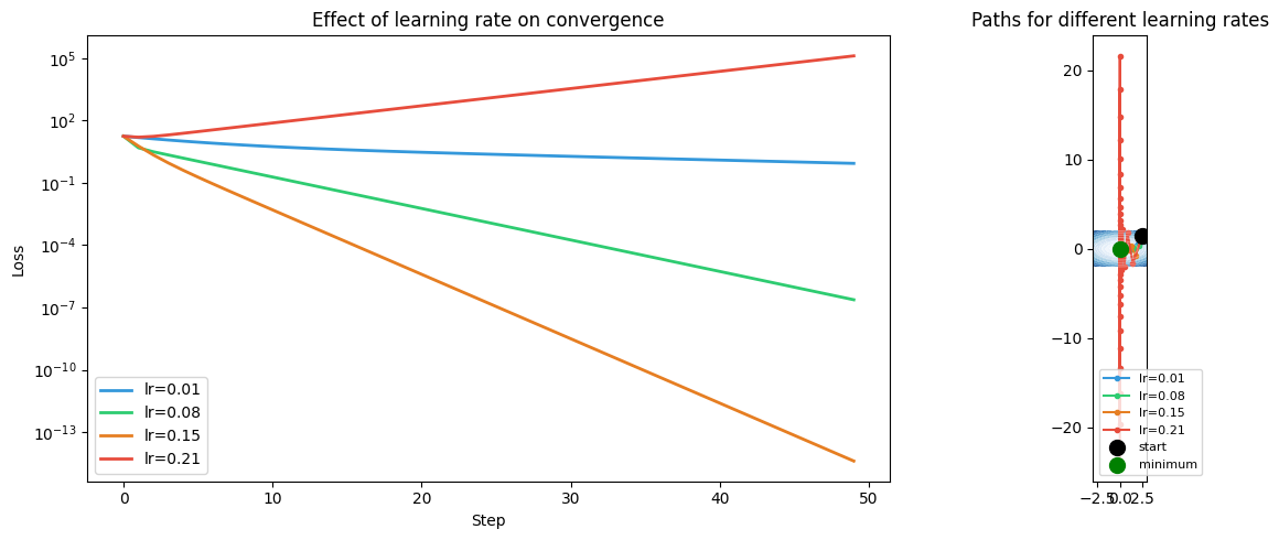
Observations:
  Too small lr → slow convergence
  Too large lr → oscillation or divergence
  Optimal lr depends on curvature of the loss surface (Hessian eigenvalues, ch217)
3. Stochastic Gradient Descent (SGD)
In practice, computing the gradient over the full dataset (batch gradient descent) is expensive. Stochastic gradient descent uses a mini-batch — a random subset of data — to estimate the gradient. The estimate is noisy but cheap.
np.random.seed(0)
N, D = 500, 2
X_full = np.random.randn(N, D)
w_true = np.array([2.0, -1.0])
y_full = X_full @ w_true + 0.5 * np.random.randn(N)

def mse_loss(w, X, y):
    return np.mean((X @ w - y)**2)

def mse_grad(w, X, y):
    residuals = X @ w - y
    return (2/len(y)) * X.T @ residuals

w0 = np.zeros(D)
lr = 0.05
n_epochs = 20
batch_size = 32

# Full batch GD
w_bgd = w0.copy()
losses_bgd = [mse_loss(w_bgd, X_full, y_full)]
for epoch in range(n_epochs * (N // batch_size)):
    g = mse_grad(w_bgd, X_full, y_full)
    w_bgd = w_bgd - lr * g
    losses_bgd.append(mse_loss(w_bgd, X_full, y_full))

# Mini-batch SGD
w_sgd = w0.copy()
losses_sgd = [mse_loss(w_sgd, X_full, y_full)]
indices = np.arange(N)
for epoch in range(n_epochs):
    np.random.shuffle(indices)
    for i in range(0, N, batch_size):
        batch = indices[i:i+batch_size]
        X_b, y_b = X_full[batch], y_full[batch]
        g = mse_grad(w_sgd, X_b, y_b)
        w_sgd = w_sgd - lr * g
        losses_sgd.append(mse_loss(w_sgd, X_full, y_full))

fig, ax = plt.subplots(figsize=(10, 5))
steps_bgd = np.linspace(0, n_epochs, len(losses_bgd))
steps_sgd = np.linspace(0, n_epochs, len(losses_sgd))
ax.semilogy(steps_bgd, losses_bgd, color='steelblue', linewidth=2, label='Full batch GD')
ax.semilogy(steps_sgd, losses_sgd, color='darkorange', linewidth=1.5, alpha=0.8, label=f'SGD (batch={batch_size})')
ax.set_xlabel('Epoch'); ax.set_ylabel('MSE Loss')
ax.set_title('Full-batch GD vs Mini-batch SGD')
ax.legend()
plt.tight_layout()
plt.show()

print(f'Batch GD final weights:   {w_bgd}')
print(f'SGD final weights:        {w_sgd}')
print(f'True weights:             {w_true}')
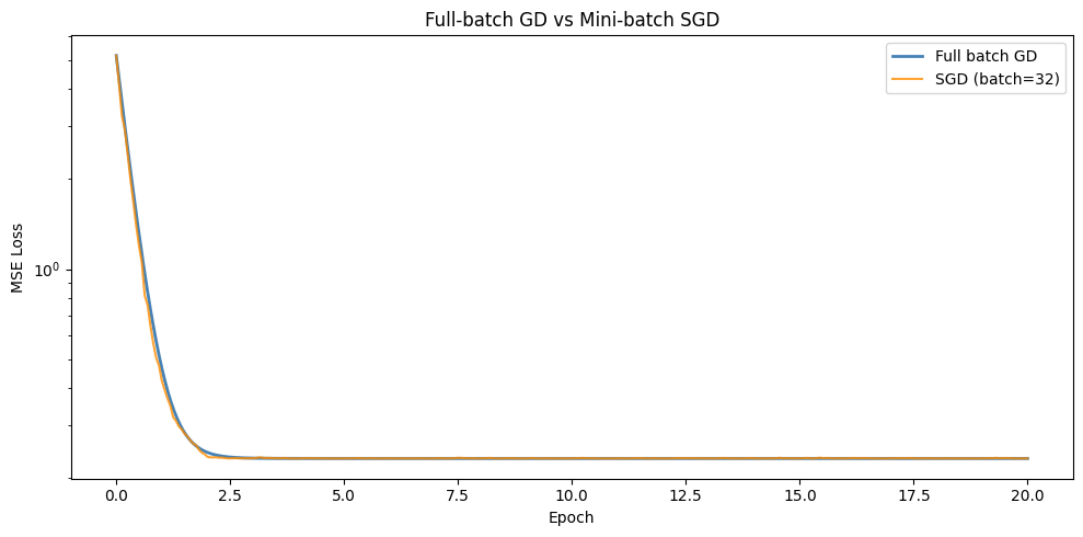
Batch GD final weights:   [ 2.03123619 -0.99509055]
SGD final weights:        [ 2.03380553 -1.00017387]
True weights:             [ 2. -1.]
4. Summary
Gradient descent: wₜ₊₁ = wₜ - η∇f(wₜ)
Learning rate η controls step size — too large oscillates, too small is slow
Convergence guaranteed for convex f with sufficiently small η
Mini-batch SGD: noisy gradient estimate, but much cheaper per step
The shape of the loss landscape (curvature) determines difficulty of optimization
5. Forward References
The difficulty of gradient descent on elongated loss surfaces motivates second-order methods discussed via the Hessian in ch217 — Second Derivatives. The optimization landscape with multiple minima and saddle points is ch213 — Optimization Landscapes and ch214 — Saddle Points. The full gradient-based learning algorithm connecting gradient descent to the chain rule is ch227 — Gradient-Based Learning.