Backpropagation is the chain rule (ch215) applied to a computation graph in reverse. It is not a new idea — it is a systematic way to accumulate gradients through nested compositions.
Every deep learning framework implements this algorithm internally. Understanding it means you understand how neural networks learn.
import numpy as np
import matplotlib.pyplot as plt

# ── Minimal scalar backprop engine ──────────────────────────────────────────
# We represent each value as a node that stores: value, gradient, and backward fn

class Value:
    def __init__(self, data, _children=(), _op=''):
        self.data = float(data)
        self.grad = 0.0
        self._backward = lambda: None
        self._prev = set(_children)
        self._op = _op

    def __repr__(self):
        return f"Value({self.data:.4f}, grad={self.grad:.4f})"

    def __add__(self, other):
        other = other if isinstance(other, Value) else Value(other)
        out = Value(self.data + other.data, (self, other), '+')
        def _backward():
            self.grad += out.grad
            other.grad += out.grad
        out._backward = _backward
        return out

    def __mul__(self, other):
        other = other if isinstance(other, Value) else Value(other)
        out = Value(self.data * other.data, (self, other), '*')
        def _backward():
            self.grad += other.data * out.grad
            other.grad += self.data * out.grad
        out._backward = _backward
        return out

    def __pow__(self, exp):
        out = Value(self.data ** exp, (self,), f'**{exp}')
        def _backward():
            self.grad += exp * (self.data ** (exp - 1)) * out.grad
        out._backward = _backward
        return out

    def relu(self):
        out = Value(max(0, self.data), (self,), 'ReLU')
        def _backward():
            self.grad += (out.data > 0) * out.grad
        out._backward = _backward
        return out

    def backward(self):
        # Topological sort
        topo, visited = [], set()
        def build(v):
            if v not in visited:
                visited.add(v)
                for child in v._prev:
                    build(child)
                topo.append(v)
        build(self)
        self.grad = 1.0
        for node in reversed(topo):
            node._backward()

print("Value class ready")
Value class ready
Forward and Backward Pass Through a Simple Network
Consider a single neuron: output = relu(w*x + b). We’ll trace both passes.
# Single neuron: out = relu(w*x + b)
# True relationship: y = 2x + 1

x = Value(2.0)   # input
w = Value(0.5)   # weight (to learn)
b = Value(0.3)   # bias   (to learn)
target = 5.0     # true output: 2*2+1=5

# Forward pass
z = w * x + b
out = z.relu()
loss = (out + Value(-target)) ** 2  # MSE loss

print(f"Forward: z={z.data:.3f}, out={out.data:.3f}, loss={loss.data:.3f}")

# Backward pass
loss.backward()
print(f"Gradients: dL/dw={w.grad:.4f}, dL/db={b.grad:.4f}")
print(f"  (Positive grads -> decrease w,b to reduce loss)")
Forward: z=1.300, out=1.300, loss=13.690
Gradients: dL/dw=-14.8000, dL/db=-7.4000
  (Positive grads -> decrease w,b to reduce loss)
Visualising Gradient Flow Through Layers
In a deep network, gradients flow backwards through every layer. The chain rule multiplies at each junction.
# Two-layer network: L = ((w2 * relu(w1*x + b1)) - target)^2
# Trace gradient magnitudes through layers

np.random.seed(42)
n_neurons = 5  # neurons per layer
x_val = 1.5

# Simulate forward pass values and backward gradients
grad_magnitudes_layer1 = []
grad_magnitudes_layer2 = []

for trial in range(100):
    w1 = np.random.randn(n_neurons) * 0.5
    b1 = np.zeros(n_neurons)
    w2 = np.random.randn(n_neurons) * 0.5
    target = 1.0

    # Forward
    h = np.maximum(0, w1 * x_val + b1)  # relu
    out = np.dot(w2, h)
    loss = (out - target) ** 2

    # Backward (manual for this structure)
    dL_dout = 2 * (out - target)
    dL_dw2 = dL_dout * h
    dL_dh = dL_dout * w2
    dL_dz = dL_dh * (h > 0)    # relu gate
    dL_dw1 = dL_dz * x_val

    grad_magnitudes_layer2.append(np.mean(np.abs(dL_dw2)))
    grad_magnitudes_layer1.append(np.mean(np.abs(dL_dw1)))

fig, ax = plt.subplots(figsize=(8, 4))
ax.hist(grad_magnitudes_layer2, bins=20, alpha=0.6, label='Layer 2 grad magnitude')
ax.hist(grad_magnitudes_layer1, bins=20, alpha=0.6, label='Layer 1 grad magnitude')
ax.set_xlabel('|gradient|'); ax.set_ylabel('Count')
ax.set_title('Gradient magnitudes: closer to output vs closer to input')
ax.legend(); ax.grid(True, alpha=0.3)
plt.tight_layout(); plt.savefig('ch216_gradients.png', dpi=100); plt.show()
print(f"Mean |grad| L2: {np.mean(grad_magnitudes_layer2):.4f}")
print(f"Mean |grad| L1: {np.mean(grad_magnitudes_layer1):.4f}")
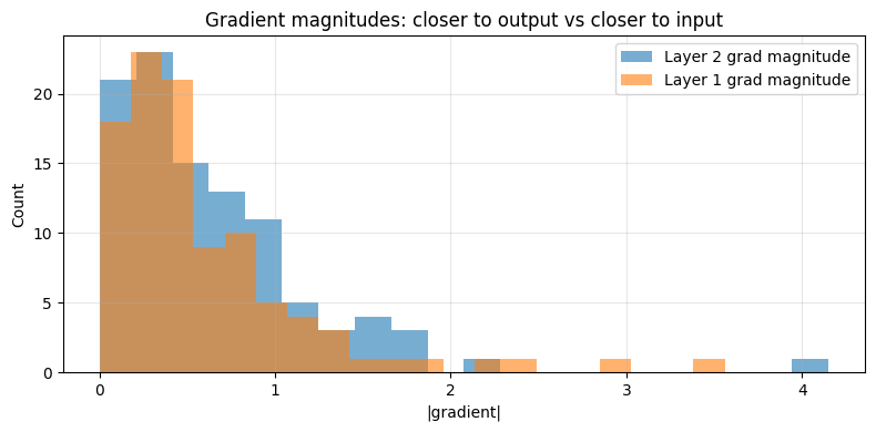
Mean |grad| L2: 0.6291
Mean |grad| L1: 0.5963
The Vanishing Gradient Problem
When gradients flow through many layers and each local derivative is < 1, the product shrinks exponentially. This makes early layers learn very slowly. It was a major obstacle in deep learning until ReLU activations and careful initialisation were adopted.
# Demonstrate vanishing gradients with sigmoid activations
def sigmoid(x): return 1 / (1 + np.exp(-x))
def sigmoid_deriv(x): s = sigmoid(x); return s * (1 - s)  # max 0.25

n_layers = 12
x_in = np.random.randn(32)  # batch of inputs
preactivations = np.random.randn(32) * 0.5  # typical preactivation values

grad = np.ones(32)  # start from output
grad_norms = [np.mean(np.abs(grad))]

for _ in range(n_layers):
    local_grad = sigmoid_deriv(preactivations)  # each element <= 0.25
    grad = grad * local_grad
    grad_norms.append(np.mean(np.abs(grad)))

fig, ax = plt.subplots(figsize=(8, 4))
ax.semilogy(grad_norms, 'o-', color='red', label='Sigmoid gradient magnitude')
ax.set_xlabel('Layer (counting backwards from output)')
ax.set_ylabel('Mean |gradient| (log scale)')
ax.set_title('Vanishing Gradients: sigmoid across 12 layers')
ax.legend(); ax.grid(True, which='both', alpha=0.3)
plt.tight_layout(); plt.savefig('ch216_vanishing.png', dpi=100); plt.show()
print(f"Gradient at layer 0: {grad_norms[0]:.4f}")
print(f"Gradient at layer 12: {grad_norms[-1]:.2e}  ({grad_norms[-1]/grad_norms[0]*100:.4f}% of original)")
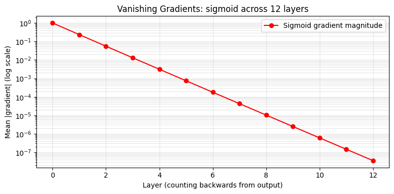
Gradient at layer 0: 1.0000
Gradient at layer 12: 3.53e-08  (0.0000% of original)
Summary
| Concept | Key Idea |
|---|---|
| Forward pass | Compute output, cache intermediate values |
| Backward pass | Apply chain rule in reverse topological order |
| Local gradient | Derivative of each op w.r.t. its inputs |
| Vanishing gradients | Repeated multiplication of small numbers shrinks signal |
Forward reference: ch228 — Project: Gradient Descent Visualizer applies this to train a small network. ch227 — Gradient-Based Learning connects the gradient signal to actual parameter updates.