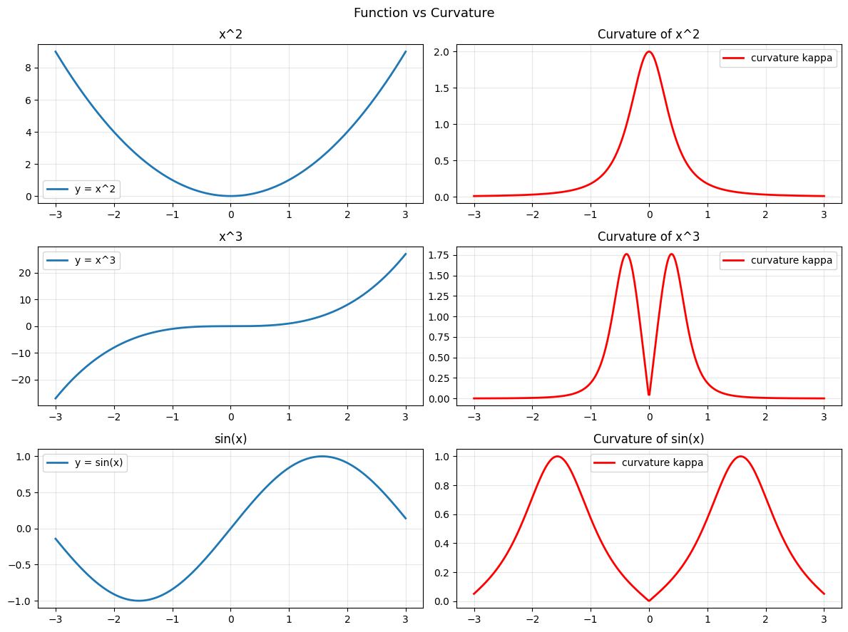
Curvature measures how fast a curve turns. A straight line has zero curvature. A tight circle has high curvature. The concept connects second derivatives (ch217) to geometry (Part IV).
In optimisation, curvature of the loss landscape determines whether gradient descent (ch212) converges quickly or oscillates.
import numpy as np
import matplotlib.pyplot as plt

# Curvature of y = f(x):
# kappa = |f''| / (1 + f'^2)^(3/2)

x = np.linspace(-3, 3, 400)

functions = [
    ('x^2',     lambda x: x**2,      lambda x: 2*x,    lambda x: 2*np.ones_like(x)),
    ('x^3',     lambda x: x**3,      lambda x: 3*x**2, lambda x: 6*x),
    ('sin(x)',   lambda x: np.sin(x), lambda x: np.cos(x), lambda x: -np.sin(x)),
]

fig, axes = plt.subplots(len(functions), 2, figsize=(12, 9))
for i, (name, f, f1, f2) in enumerate(functions):
    kappa = np.abs(f2(x)) / (1 + f1(x)**2) ** 1.5
    axes[i, 0].plot(x, f(x), lw=2, label=f'y = {name}')
    axes[i, 0].set_title(f'{name}'); axes[i, 0].legend(); axes[i, 0].grid(True, alpha=0.3)
    axes[i, 1].plot(x, kappa, lw=2, color='red', label='curvature kappa')
    axes[i, 1].set_title(f'Curvature of {name}'); axes[i, 1].legend(); axes[i, 1].grid(True, alpha=0.3)

plt.suptitle('Function vs Curvature', fontsize=13)
plt.tight_layout(); plt.savefig('ch218_curvature.png', dpi=100); plt.show()
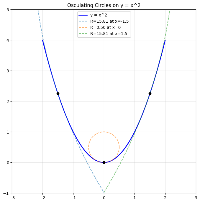
Radius of Curvature
At each point on a curve, we can fit the osculating circle — the circle that best approximates the curve at that point. Its radius R = 1/kappa is the radius of curvature.
# Osculating circles at different points on y = x^2
fig, ax = plt.subplots(figsize=(8, 7))
x_curve = np.linspace(-2, 2, 400)
ax.plot(x_curve, x_curve**2, 'b', lw=2, label='y = x^2')
ax.set_aspect('equal')

for x0 in [-1.5, 0, 1.5]:
    y0 = x0**2
    f1_at = 2*x0
    f2_at = 2.0
    kappa = abs(f2_at) / (1 + f1_at**2)**1.5
    R = 1.0 / kappa

    # Centre of osculating circle
    cx = x0 - f1_at * (1 + f1_at**2) / f2_at
    cy = y0 + (1 + f1_at**2) / f2_at

    theta = np.linspace(0, 2*np.pi, 200)
    ax.plot(cx + R*np.cos(theta), cy + R*np.sin(theta), '--', alpha=0.6, label=f'R={R:.2f} at x={x0}')
    ax.plot(x0, y0, 'ko', ms=6)

ax.legend(loc='upper center'); ax.grid(True, alpha=0.3)
ax.set_xlim(-3, 3); ax.set_ylim(-1, 5)
ax.set_title('Osculating Circles on y = x^2')
plt.tight_layout(); plt.savefig('ch218_osculating.png', dpi=100); plt.show()
Curvature in Optimisation
High curvature means the gradient changes rapidly — gradient steps that are calibrated for one point will overshoot. Low curvature means slow progress. The condition number of the Hessian captures this imbalance across dimensions.
# Loss landscape with different curvatures in each direction
# L = a*x^2 + b*y^2  with a >> b => ill-conditioned

x_g = np.linspace(-2, 2, 100)
y_g = np.linspace(-2, 2, 100)
X, Y = np.meshgrid(x_g, y_g)

fig, axes = plt.subplots(1, 2, figsize=(12, 5))
for ax, (a, b), title in zip(axes,
        [(1, 1), (10, 0.1)],
        ['Well-conditioned (a=b=1)', 'Ill-conditioned (a=10, b=0.1)']):
    Z = a * X**2 + b * Y**2
    ax.contour(X, Y, Z, levels=15, cmap='viridis')
    ax.set_aspect('equal'); ax.set_title(title)
    ax.set_xlabel('x'); ax.set_ylabel('y')

plt.suptitle('Curvature Imbalance and Optimisation Difficulty')
plt.tight_layout(); plt.savefig('ch218_conditioning.png', dpi=100); plt.show()
print("Condition number (a=10, b=0.1):", 10 / 0.1)
print("Gradient descent struggles when this ratio is large.")
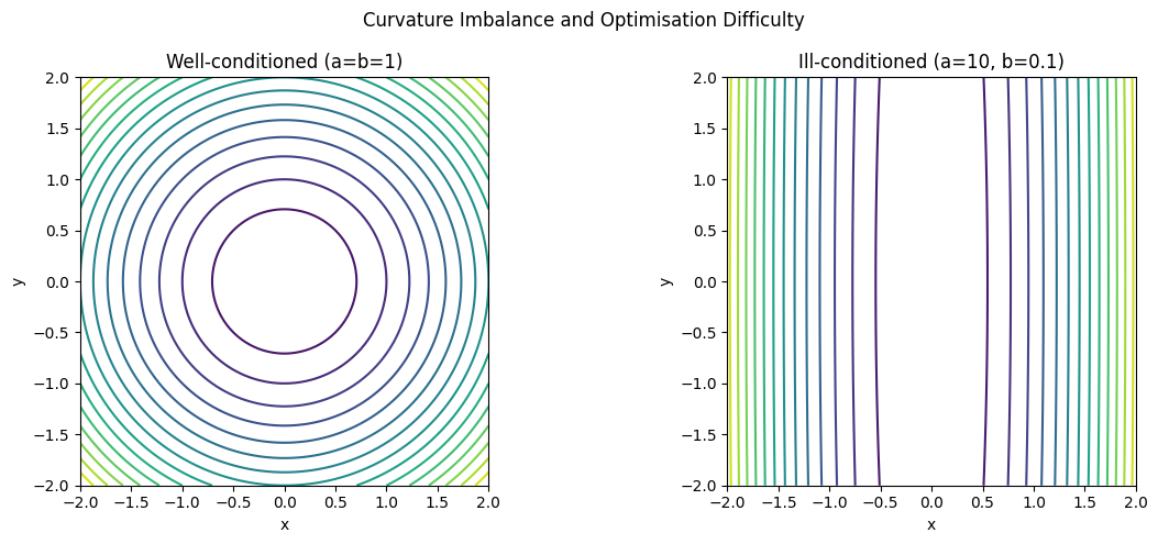
Condition number (a=10, b=0.1): 100.0
Gradient descent struggles when this ratio is large.
Summary
| Concept | Formula / Meaning |
|---|---|
| Curvature | kappa = |
| Radius of curvature | R = 1/kappa |
| Osculating circle | Circle with radius R tangent to curve |
| Condition number | max eigenvalue / min eigenvalue of Hessian |
Forward reference: ch219 — Taylor Series uses curvature (the second-order term) to approximate functions near a point.