If differentiation is about instantaneous rates of change, integration is about accumulation over an interval. The integral of a rate is a total. Distance is the integral of velocity. Area is the integral of height.
The central idea: chop the interval into many thin pieces, sum up the contributions of each piece, take the limit as the pieces shrink to zero.
import numpy as np
import matplotlib.pyplot as plt

# Visual: approximating the area under f(x) = x^2 from 0 to 2
# True integral = [x^3/3] from 0 to 2 = 8/3 ≈ 2.667

def f(x): return x**2

a, b = 0, 2
exact = b**3/3 - a**3/3

fig, axes = plt.subplots(1, 3, figsize=(13, 4))
x_smooth = np.linspace(a, b, 300)

for ax, n in zip(axes, [4, 10, 50]):
    x_bars = np.linspace(a, b, n+1)
    heights = f(x_bars[:-1])  # left Riemann sum
    width = (b - a) / n
    approx = np.sum(heights) * width

    ax.fill_between(x_smooth, f(x_smooth), alpha=0.1, color='blue')
    ax.bar(x_bars[:-1], heights, width=width, align='edge', alpha=0.5,
           color='orange', edgecolor='black', linewidth=0.5)
    ax.plot(x_smooth, f(x_smooth), 'b', lw=2)
    ax.set_title(f'n={n} strips\nApprox={approx:.4f}, Exact={exact:.4f}')
    ax.set_xlabel('x'); ax.set_ylabel('f(x)')

plt.suptitle('Riemann Sum Approximation of Area Under x²')
plt.tight_layout(); plt.savefig('ch221_riemann.png', dpi=100); plt.show()
print(f"Exact integral: {exact:.6f}")
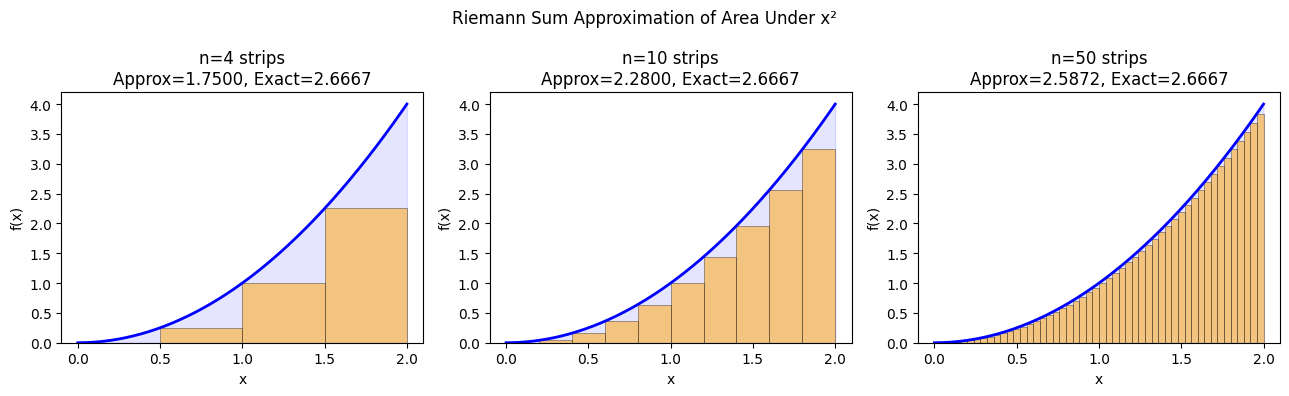
Exact integral: 2.666667
The Fundamental Theorem of Calculus
The FTC unifies differentiation and integration — they are inverse operations:
If
F'(x) = f(x), then the integral of f from a to b equalsF(b) - F(a).If
G(x) = integral from a to x of f(t) dt, thenG'(x) = f(x).
This is why the antiderivative is also called the indefinite integral.
# Demonstrate FTC numerically: integrate sin(x), get -cos(x)
# F(x) = integral of sin from 0 to x = -cos(x) + cos(0) = 1 - cos(x)

x_vals = np.linspace(0, 2*np.pi, 300)
h = x_vals[1] - x_vals[0]

# Numerical cumulative integral using cumulative sum (left Riemann)
f_vals = np.sin(x_vals)
F_numerical = np.cumsum(f_vals) * h

# Analytical: -cos(x) + 1
F_analytical = 1 - np.cos(x_vals)

# Derivative of F should give back sin(x)
dF_dx_numerical = np.gradient(F_analytical, x_vals)

fig, axes = plt.subplots(1, 2, figsize=(12, 4))
axes[0].plot(x_vals, F_analytical, lw=2, label='F(x) = 1 - cos(x) [analytical]')
axes[0].plot(x_vals, F_numerical, '--', lw=1.5, label='F(x) [numerical cumsum]')
axes[0].set_title('Integral of sin(x)'); axes[0].legend(); axes[0].grid(True, alpha=0.3)

axes[1].plot(x_vals, np.sin(x_vals), lw=2, label='sin(x) [original]')
axes[1].plot(x_vals, dF_dx_numerical, '--', lw=1.5, label="F'(x) [numerical]")
axes[1].set_title("Derivative of F recovers sin(x)"); axes[1].legend(); axes[1].grid(True, alpha=0.3)

plt.suptitle('Fundamental Theorem of Calculus — Numerical Verification')
plt.tight_layout(); plt.savefig('ch221_ftc.png', dpi=100); plt.show()
print(f"Max error (integral): {np.max(np.abs(F_numerical - F_analytical)):.4f}")
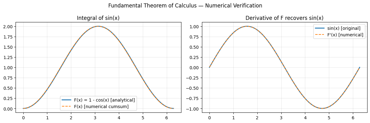
Max error (integral): 0.0105
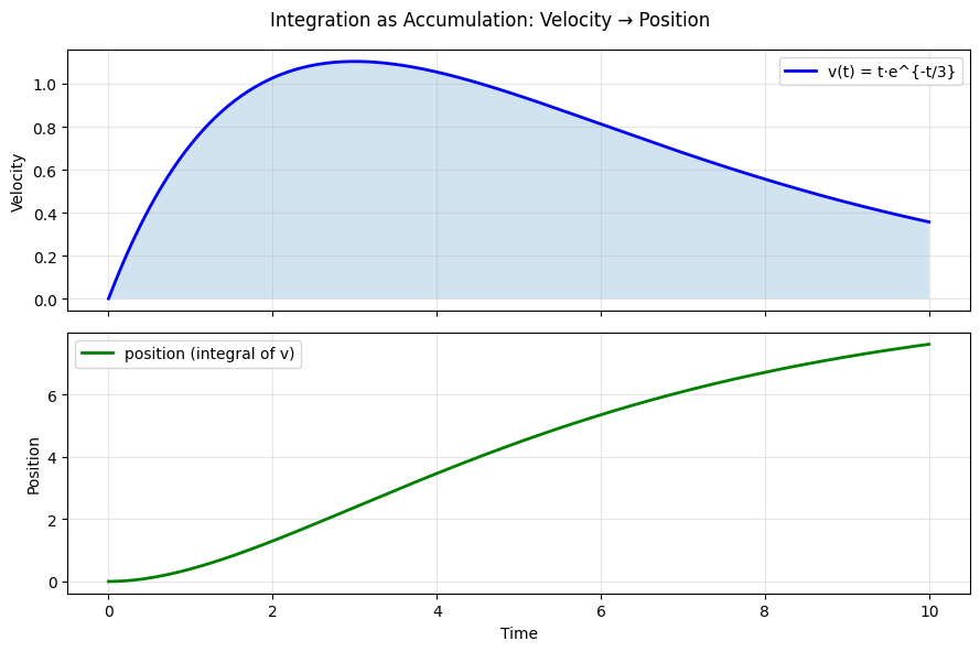
Integration as Accumulation
Integration is not just area — it is the general tool for accumulation:
| Physical quantity | Rate (derivative) | Accumulated total (integral) |
|---|---|---|
| Distance | Velocity | Position |
| Position | Acceleration | Velocity |
| Revenue | Revenue rate | Total revenue |
| Probability | CDF | |
| Energy | Power | Work |
# Real example: position from velocity
# v(t) = t * exp(-t/3)  (accelerates then decelerates)
t = np.linspace(0, 10, 500)
v = t * np.exp(-t/3)

# True position: integral using scipy
from scipy.integrate import cumulative_trapezoid
position = cumulative_trapezoid(v, t, initial=0)

fig, axes = plt.subplots(2, 1, figsize=(9, 6), sharex=True)
axes[0].plot(t, v, color='blue', lw=2, label='v(t) = t·e^{-t/3}')
axes[0].fill_between(t, v, alpha=0.2)
axes[0].set_ylabel('Velocity'); axes[0].legend(); axes[0].grid(True, alpha=0.3)
axes[1].plot(t, position, color='green', lw=2, label='position (integral of v)')
axes[1].set_ylabel('Position'); axes[1].set_xlabel('Time')
axes[1].legend(); axes[1].grid(True, alpha=0.3)
plt.suptitle('Integration as Accumulation: Velocity → Position')
plt.tight_layout(); plt.savefig('ch221_accumulation.png', dpi=100); plt.show()
Summary
| Concept | Key Idea |
|---|---|
| Riemann sum | Approximate area with rectangles, refine limit |
| FTC part 1 | Evaluate definite integral via antiderivative |
| FTC part 2 | Differentiate a cumulative integral → original function |
| Integration as accumulation | Applies far beyond area: distance, probability, energy |
Forward reference: ch222 — Area Under Curve extends to signed areas and probability density functions. ch223 — Numerical Integration implements efficient algorithms beyond Riemann sums.