0. Overview
Problem statement: Gradient descent is the engine of all learned models. But watching a loss curve decline tells you little about why it behaves as it does — why certain learning rates diverge, why momentum helps in ravines, why Adam adapts. This project builds a self-contained visualizer that makes the geometry of gradient descent legible.
Concepts applied:
Gradient computation and backpropagation (ch209, ch216)
Gradient descent variants (ch212, ch227)
Optimization landscapes: saddle points, ravines (ch213, ch214)
Taylor series: quadratic approximation of loss (ch219)
Expected output: Animated trajectory plots on several 2D loss surfaces, with side-by-side optimizer comparison.
Difficulty: Intermediate. Estimated time: 60–90 min.
import numpy as np
import matplotlib.pyplot as plt
import matplotlib.animation as animation
from IPython.display import HTML

np.random.seed(42)
print("Setup complete.")
Setup complete.
1. Setup — Loss Surface Library
# Define a set of canonical 2D loss surfaces for visualisation

def quadratic(w):
    w1, w2 = w
    return (w1 - 1)**2 + 5*(w2 - 1)**2

def grad_quadratic(w):
    w1, w2 = w
    return np.array([2*(w1 - 1), 10*(w2 - 1)])

def rosenbrock(w):
    x, y = w
    return (1 - x)**2 + 100*(y - x**2)**2

def grad_rosenbrock(w):
    x, y = w
    dx = -2*(1 - x) - 400*x*(y - x**2)
    dy = 200*(y - x**2)
    return np.array([dx, dy])

def saddle(w):
    x, y = w
    return x**2 - y**2

def grad_saddle(w):
    x, y = w
    return np.array([2*x, -2*y])

surfaces = {
    'Quadratic (ideal)': (quadratic, grad_quadratic, [2.5, 2.5], (-0.5, 3.5), (-0.5, 3.5)),
    'Rosenbrock (valley)': (rosenbrock, grad_rosenbrock, [-1.0, 2.0], (-2, 2), (-0.5, 3.5)),
    'Saddle Point': (saddle, grad_saddle, [1.5, 0.1], (-2.5, 2.5), (-2.5, 2.5)),
}
print("Loss surfaces defined:", list(surfaces.keys()))
Loss surfaces defined: ['Quadratic (ideal)', 'Rosenbrock (valley)', 'Saddle Point']
2. Stage 1 — Optimizer Implementations
class OptimizerBase:
    def __init__(self, lr):
        self.lr = lr
        self.state = {}

    def step(self, w, grad):
        raise NotImplementedError

class SGD(OptimizerBase):
    def step(self, w, grad):
        return w - self.lr * grad

class MomentumSGD(OptimizerBase):
    def __init__(self, lr, mu=0.9):
        super().__init__(lr); self.mu = mu
    def step(self, w, grad):
        v = self.state.get('v', np.zeros_like(w))
        v = self.mu * v + grad
        self.state['v'] = v
        return w - self.lr * v

class Adam(OptimizerBase):
    def __init__(self, lr=0.1, beta1=0.9, beta2=0.999, eps=1e-8):
        super().__init__(lr)
        self.beta1, self.beta2, self.eps = beta1, beta2, eps
    def step(self, w, grad):
        t  = self.state.get('t', 0) + 1
        m  = self.beta1 * self.state.get('m', np.zeros_like(w)) + (1 - self.beta1) * grad
        v  = self.beta2 * self.state.get('v', np.zeros_like(w)) + (1 - self.beta2) * grad**2
        self.state.update({'t': t, 'm': m, 'v': v})
        m_hat = m / (1 - self.beta1**t)
        v_hat = v / (1 - self.beta2**t)
        return w - self.lr * m_hat / (np.sqrt(v_hat) + self.eps)

def run_optimizer(opt, grad_fn, w0, n_steps=200):
    w = w0.copy().astype(float)
    path = [w.copy()]
    for _ in range(n_steps):
        g = grad_fn(w)
        w = opt.step(w, g)
        path.append(w.copy())
    return np.array(path)

print("Optimizers: SGD, MomentumSGD, Adam")
Optimizers: SGD, MomentumSGD, Adam
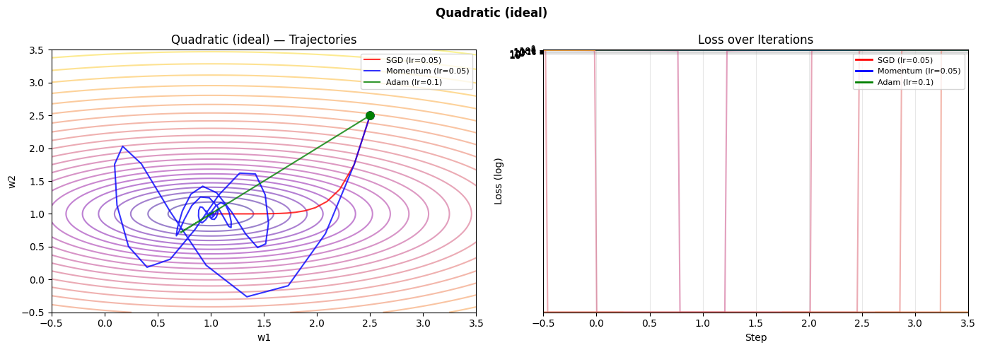
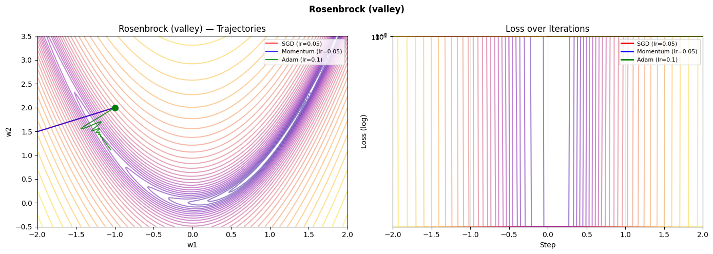
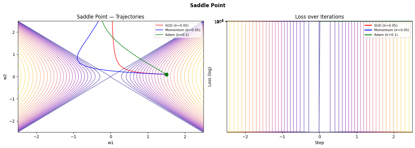
3. Stage 2 — Trajectory Visualisation
def plot_trajectories(surface_name, n_steps=150, n_contours=30):
    loss_fn, grad_fn, w0, xlim, ylim = surfaces[surface_name]

    # Build contour grid
    xs = np.linspace(*xlim, 200)
    ys = np.linspace(*ylim, 200)
    X, Y = np.meshgrid(xs, ys)
    Z = np.vectorize(lambda x, y: loss_fn([x, y]))(X, Y)
    Z_log = np.log1p(np.clip(Z, 0, None))  # log scale for better visual

    optimizers = {
        'SGD (lr=0.05)':          SGD(lr=0.05),
        'Momentum (lr=0.05)':     MomentumSGD(lr=0.05),
        'Adam (lr=0.1)':          Adam(lr=0.1),
    }
    colors = ['red', 'blue', 'green']

    fig, axes = plt.subplots(1, 2, figsize=(14, 5))
    for ax in axes:
        ax.contour(X, Y, Z_log, levels=n_contours, cmap='plasma', alpha=0.5)
        ax.set_xlim(xlim); ax.set_ylim(ylim)
        ax.set_xlabel('w1'); ax.set_ylabel('w2')

    axes[0].set_title(f'{surface_name} — Trajectories')
    axes[1].set_title('Loss over Iterations')

    for (name, opt), color in zip(optimizers.items(), colors):
        path = run_optimizer(opt, grad_fn, np.array(w0), n_steps)
        losses = [loss_fn(w) for w in path]
        axes[0].plot(path[:, 0], path[:, 1], '-', color=color, lw=1.5, alpha=0.8, label=name)
        axes[0].plot(path[0, 0], path[0, 1], 'o', color=color, ms=8)
        axes[1].semilogy(losses, color=color, lw=2, label=name)

    axes[0].legend(fontsize=8); axes[1].legend(fontsize=8)
    axes[1].set_xlabel('Step'); axes[1].set_ylabel('Loss (log)')
    axes[1].grid(True, which='both', alpha=0.3)
    plt.suptitle(surface_name, fontsize=12, fontweight='bold')
    plt.tight_layout()
    plt.savefig(f"ch228_{surface_name.replace(' ', '_').replace('(', '').replace(')', '')}.png", dpi=100)
    plt.show()

for name in surfaces:
    plot_trajectories(name)
C:\Users\user\AppData\Local\Temp\ipykernel_24116\2162303551.py:17: RuntimeWarning: overflow encountered in scalar power
  dx = -2*(1 - x) - 400*x*(y - x**2)
C:\Users\user\AppData\Local\Temp\ipykernel_24116\2162303551.py:18: RuntimeWarning: overflow encountered in scalar power
  dy = 200*(y - x**2)
C:\Users\user\AppData\Local\Temp\ipykernel_24116\2162303551.py:17: RuntimeWarning: invalid value encountered in scalar subtract
  dx = -2*(1 - x) - 400*x*(y - x**2)
C:\Users\user\AppData\Local\Temp\ipykernel_24116\2162303551.py:18: RuntimeWarning: invalid value encountered in scalar subtract
  dy = 200*(y - x**2)
C:\Users\user\AppData\Local\Temp\ipykernel_24116\2162303551.py:13: RuntimeWarning: overflow encountered in scalar power
  return (1 - x)**2 + 100*(y - x**2)**2
C:\Users\user\AppData\Local\Temp\ipykernel_24116\2162303551.py:13: RuntimeWarning: invalid value encountered in scalar subtract
  return (1 - x)**2 + 100*(y - x**2)**2
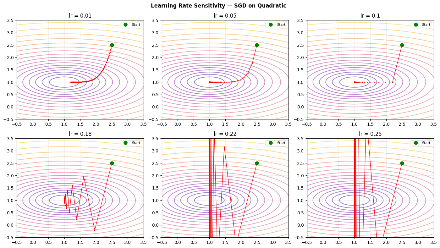
4. Stage 3 — Learning Rate Sensitivity Study
# How does learning rate affect convergence on a simple quadratic?
loss_fn, grad_fn, w0_quad, xlim, ylim = surfaces['Quadratic (ideal)']

lr_values = [0.01, 0.05, 0.1, 0.18, 0.22, 0.25]
n_steps = 100

fig, axes = plt.subplots(2, 3, figsize=(14, 8))
xs = np.linspace(*xlim, 200)
ys = np.linspace(*ylim, 200)
X, Y = np.meshgrid(xs, ys)
Z = np.vectorize(lambda x, y: loss_fn([x, y]))(X, Y)

for ax, lr in zip(axes.flat, lr_values):
    ax.contour(X, Y, np.log1p(Z), levels=20, cmap='plasma', alpha=0.5)
    path = run_optimizer(SGD(lr=lr), grad_fn, np.array(w0_quad), n_steps)
    ax.plot(path[:, 0], path[:, 1], 'r.-', ms=3, lw=1)
    ax.plot(path[0, 0], path[0, 1], 'go', ms=8, label='Start')
    ax.set_title(f'lr = {lr}'); ax.set_xlim(xlim); ax.set_ylim(ylim)
    ax.legend(fontsize=8); ax.grid(True, alpha=0.2)

plt.suptitle('Learning Rate Sensitivity — SGD on Quadratic', fontsize=12, fontweight='bold')
plt.tight_layout(); plt.savefig('ch228_lr_sensitivity.png', dpi=100); plt.show()
5. Results & Reflection
What was built: A trajectory visualizer that shows gradient descent paths on three canonical loss surfaces — a well-conditioned quadratic, the notoriously difficult Rosenbrock valley, and a saddle point.
What math made it possible:
Gradients (ch209) give the direction of steepest ascent at each point
The chain rule (ch215) lets us compute those gradients analytically
Momentum and Adam (ch227) accumulate gradient history to overcome oscillation
Quadratic approximation (ch219) explains why learning rate > 2/L causes divergence
Extension challenges:
Add Nesterov momentum (look-ahead gradient evaluation) and compare its path on the Rosenbrock surface to standard momentum.
Implement a learning rate scheduler (e.g., cosine annealing) and observe its effect on final convergence.
Add a 3D surface plot that rotates in sync with the 2D trajectory animation.