Part VIII: Probability | Computational Mathematics for Programmers
1. The Problem
You have a prior belief. You observe evidence. How should you update your belief?
Bayes’ theorem answers this precisely. It is not a heuristic or a metaphor — it is an algebraic consequence of the definition of conditional probability (introduced in ch245).
2. Derivation from First Principles
From the multiplication rule (ch245):
Both expressions equal P(A ∩ B). Set them equal:
Solve for P(A|B):
In the context of belief updating:
A = hypothesis (e.g., “email is spam”)
B = observed evidence (e.g., “email contains ‘offer’”)
P(A) = prior — your belief before seeing evidence
P(B|A) = likelihood — probability of evidence given the hypothesis
P(B) = marginal likelihood — probability of evidence under any hypothesis
P(A|B) = posterior — updated belief after evidence
import numpy as np
import matplotlib.pyplot as plt

def bayes_update(prior: float, likelihood: float, p_evidence: float) -> float:
    """
    Compute posterior P(H|E) given:
      prior      = P(H)
      likelihood = P(E|H)
      p_evidence = P(E) — marginal probability of evidence
    """
    return (likelihood * prior) / p_evidence


# Spam filter from the Part VIII intro
p_spam = 0.30              # P(spam)
p_legit = 1 - p_spam       # P(legit)
p_offer_given_spam = 0.40  # P('offer' | spam)
p_offer_given_legit = 0.05 # P('offer' | legit)

# Law of total probability: P('offer') = P('offer'|spam)P(spam) + P('offer'|legit)P(legit)
p_offer = p_offer_given_spam * p_spam + p_offer_given_legit * p_legit

# Bayes' theorem
p_spam_given_offer = bayes_update(p_spam, p_offer_given_spam, p_offer)

print("Spam Filter — Bayes' Theorem")
print(f"  Prior P(spam) = {p_spam:.4f}")
print(f"  P('offer' | spam) = {p_offer_given_spam:.4f}")
print(f"  P('offer' | legit) = {p_offer_given_legit:.4f}")
print(f"  P('offer') = {p_offer:.4f}  [law of total probability]")
print(f"  Posterior P(spam | 'offer') = {p_spam_given_offer:.4f}")
Spam Filter — Bayes' Theorem
Prior P(spam) = 0.3000
P('offer' | spam) = 0.4000
P('offer' | legit) = 0.0500
P('offer') = 0.1550 [law of total probability]
Posterior P(spam | 'offer') = 0.7742
The prior was 30% spam. Observing “offer” shifts the posterior to 77.4%. The word carries strong evidence because it is 8× more common in spam than in legitimate mail.
3. The Full Form With a Partition
When H and Hᶜ partition Ω, the denominator P(B) can always be expanded using the law of total probability:
This form is self-contained — you never need to know P(E) directly.
def bayes_two_class(prior_h: float, likelihood_h: float, likelihood_not_h: float) -> float:
    """
    P(H|E) using full Bayes with expanded denominator.
    No need to pre-compute P(E).
    """
    numerator = likelihood_h * prior_h
    denominator = likelihood_h * prior_h + likelihood_not_h * (1 - prior_h)
    return numerator / denominator


# Medical test example
# Disease prevalence: 1%
# Test sensitivity (true positive rate): 99%
# Test specificity (true negative rate): 95% → false positive rate: 5%

prior_disease = 0.01
sensitivity = 0.99   # P(positive | disease)
false_positive = 0.05  # P(positive | no disease)

posterior = bayes_two_class(prior_disease, sensitivity, false_positive)

print("Medical Test Example")
print(f"  Disease prevalence: {prior_disease:.0%}")
print(f"  Test sensitivity: {sensitivity:.0%}")
print(f"  False positive rate: {false_positive:.0%}")
print(f"  P(disease | positive test) = {posterior:.4f} ({posterior:.1%})")
print()
print("  Despite 99% sensitivity, a positive test on a low-prevalence")
print(f"  disease means only {posterior:.1%} chance of actually having it.")
print("  This is the base rate fallacy — Bayes corrects for it.")
Medical Test Example
Disease prevalence: 1%
Test sensitivity: 99%
False positive rate: 5%
P(disease | positive test) = 0.1667 (16.7%)
Despite 99% sensitivity, a positive test on a low-prevalence
disease means only 16.7% chance of actually having it.
This is the base rate fallacy — Bayes corrects for it.
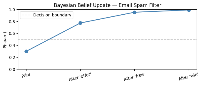
4. Bayesian Updating Sequentially
Each posterior becomes the next prior. Evidence accumulates.
# Sequential Bayesian updating
# Each email is independently scanned for spam words.
# Words: 'offer', 'free', 'win'

likelihoods_spam  = {'offer': 0.40, 'free': 0.60, 'win': 0.50}
likelihoods_legit = {'offer': 0.05, 'free': 0.10, 'win': 0.08}

def sequential_bayes(prior, words_found):
    posterior = prior
    history = [prior]
    for word in words_found:
        posterior = bayes_two_class(
            posterior,
            likelihoods_spam[word],
            likelihoods_legit[word]
        )
        history.append(posterior)
    return posterior, history

words = ['offer', 'free', 'win']
final_p, history = sequential_bayes(prior=0.30, words_found=words)

print("Sequential updates after each spam word:")
labels = ['Prior'] + [f"After '{w}'" for w in words]
for label, p in zip(labels, history):
    bar = '█' * int(p * 40)
    print(f"  {label:<18}: {p:.4f}  {bar}")

# Plot
fig, ax = plt.subplots(figsize=(7, 3))
ax.plot(range(len(history)), history, 'o-', color='steelblue', linewidth=2, markersize=8)
ax.axhline(0.5, color='gray', linestyle='--', alpha=0.5, label='Decision boundary')
ax.set_xticks(range(len(history)))
ax.set_xticklabels(labels, rotation=15)
ax.set_ylabel('P(spam)')
ax.set_title('Bayesian Belief Update — Email Spam Filter')
ax.set_ylim(0, 1)
ax.legend()
plt.tight_layout()
plt.show()
Sequential updates after each spam word:
Prior : 0.3000 ████████████
After 'offer' : 0.7742 ██████████████████████████████
After 'free' : 0.9536 ██████████████████████████████████████
After 'win' : 0.9923 ███████████████████████████████████████
5. Bayes’ Theorem in Machine Learning
Every probabilistic ML model applies Bayes’ theorem:
Naive Bayes classifier: assumes features are independent given class, factoring the likelihood.
Bayesian neural networks: place priors on weights, compute posterior distributions.
Kalman filter: sequential Bayesian updates for state estimation.
A/B testing: update beliefs about conversion rates as data accumulates (see ch286).
# Minimal Naive Bayes classifier from scratch
# Training data: (word_count_offer, label)

class NaiveBayesBinaryClassifier:
    """Naive Bayes for binary classification from counts."""

    def __init__(self):
        self.prior = {}
        self.likelihoods = {}  # {class: {feature: P(feature|class)}}

    def fit(self, X, y, feature_names):
        """
        X: shape (n_samples, n_features) — binary feature presence
        y: labels (0 or 1)
        """
        X, y = np.array(X), np.array(y)
        classes = np.unique(y)
        n = len(y)

        for c in classes:
            mask = y == c
            self.prior[c] = mask.sum() / n
            # Laplace smoothing: add 1 to numerator and denominator
            self.likelihoods[c] = {
                feat: (X[mask, i].sum() + 1) / (mask.sum() + 2)
                for i, feat in enumerate(feature_names)
            }
        self.feature_names = feature_names
        return self

    def predict_proba(self, x, feature_names):
        """Return P(class=1 | x) using Bayes' theorem."""
        scores = {}
        for c, prior in self.prior.items():
            log_prob = np.log(prior)
            for i, feat in enumerate(feature_names):
                p = self.likelihoods[c][feat]
                log_prob += np.log(p) if x[i] == 1 else np.log(1 - p)
            scores[c] = log_prob
        # Convert log-probabilities to normalized probabilities
        max_log = max(scores.values())
        exp_scores = {c: np.exp(v - max_log) for c, v in scores.items()}
        total = sum(exp_scores.values())
        return {c: v / total for c, v in exp_scores.items()}


# Tiny dataset: [has_offer, has_free, has_win] → spam(1) or legit(0)
features = ['offer', 'free', 'win']
X_train = [
    [1, 1, 0],  # spam
    [1, 0, 1],  # spam
    [0, 1, 1],  # spam
    [0, 0, 0],  # legit
    [1, 0, 0],  # legit
    [0, 0, 0],  # legit
]
y_train = [1, 1, 1, 0, 0, 0]

clf = NaiveBayesBinaryClassifier().fit(X_train, y_train, features)

# Predict a new email: contains 'offer' and 'free'
x_new = [1, 1, 0]
proba = clf.predict_proba(x_new, features)
print(f"New email [offer=1, free=1, win=0]:")
print(f"  P(spam | features) = {proba[1]:.4f}")
print(f"  P(legit | features) = {proba[0]:.4f}")
New email [offer=1, free=1, win=0]:
P(spam | features) = 0.6923
P(legit | features) = 0.3077
6. Summary
Bayes’ theorem follows directly from the definition of conditional probability — it is not a separate axiom.
P(H|E) = P(E|H)·P(H) / P(E): posterior = likelihood × prior / evidence.
The denominator P(E) normalizes the result and can be expanded using the law of total probability.
Sequential updating: each posterior becomes the prior for the next observation.
Every probabilistic classifier is an implementation of Bayes’ theorem.
7. Forward References
Bayes’ theorem is the backbone of Part IX. It reappears in ch287 (Bayesian Statistics) as a framework for full probabilistic inference, and the prior/posterior distinction drives Bayesian model selection. The likelihood function P(E|H) is formalized through the distributions in ch248–ch253.