ch272 — Data Cleaning - Mathematics for Programmers

(Building on ch271 — Data and Measurement: measurement error is the root cause of most data quality problems.)

1. Why Cleaning Matters¶

Garbage in, garbage out is not a metaphor. It is a mathematical fact: every estimator, test, and model assumes the input data meets certain conditions. When those conditions are violated — missing values, duplicates, outliers, inconsistent encoding — the estimator’s guarantees break down.

Data cleaning is not preprocessing. It is the act of constructing a dataset whose properties match the assumptions of the analysis you intend to run.

2. The Five Classes of Data Problems¶

Problem	Definition	Effect on analysis
Missing values	NaN, None, sentinel values	Biases estimates if not missing completely at random
Duplicates	Identical or near-identical rows	Inflates sample size, biases toward repeated records
Outliers	Extreme values relative to the distribution	Distorts mean, regression coefficients, covariance
Encoding inconsistency	‘US’, ‘usa’, ‘United States’ as three categories	Creates spurious categories, reduces effective N
Type errors	‘42.5’ stored as string	Prevents arithmetic; produces silent errors

3. Setup: A Deliberately Dirty Dataset¶

import numpy as np
import matplotlib.pyplot as plt

rng = np.random.default_rng(42)
n = 200

# Ground truth
age      = rng.integers(18, 65, size=n).astype(float)
revenue  = 50 + 3 * age + rng.normal(0, 20, n)  # linear relationship + noise
country  = rng.choice(['US', 'UK', 'DE', 'FR'], n)

# --- Inject problems ---

# 1. Missing values (10%)
missing_age = rng.choice(n, 20, replace=False)
missing_rev = rng.choice(n, 20, replace=False)
age[missing_age] = np.nan
revenue[missing_rev] = np.nan

# 2. Outliers: a few extreme revenue values
outlier_idx = rng.choice(n, 5, replace=False)
revenue[outlier_idx] = rng.uniform(2000, 5000, 5)

# 3. Duplicates: copy 10 rows
dup_idx = rng.choice(n, 10, replace=False)
age_full    = np.concatenate([age,    age[dup_idx]])
revenue_full = np.concatenate([revenue, revenue[dup_idx]])
country_full = np.concatenate([country, country[dup_idx]])

# 4. Encoding inconsistency
raw_country = country_full.copy()
fix_idx = rng.choice(len(raw_country), 15, replace=False)
raw_country[fix_idx[:5]]   = 'us'
raw_country[fix_idx[5:10]] = 'United States'
raw_country[fix_idx[10:]]  = ' DE'

print(f"Raw dataset: {len(age_full)} rows (includes {10} duplicates)")
print(f"Missing age: {np.isnan(age_full).sum()}")
print(f"Missing revenue: {np.isnan(revenue_full).sum()}")
print(f"Outlier revenue values (>500): {np.sum(revenue_full[~np.isnan(revenue_full)] > 500)}")
unique, counts = np.unique(raw_country, return_counts=True)
print(f"\nRaw country encoding: {dict(zip(unique, counts))}")

Raw dataset: 210 rows (includes 10 duplicates)
Missing age: 21
Missing revenue: 22
Outlier revenue values (>500): 5

Raw country encoding: {np.str_(' D'): np.int64(5), np.str_('DE'): np.int64(54), np.str_('FR'): np.int64(50), np.str_('UK'): np.int64(46), np.str_('US'): np.int64(45), np.str_('Un'): np.int64(5), np.str_('us'): np.int64(5)}

4. Handling Missing Values¶

Three mechanisms govern missingness — the choice of handling method depends on which applies:

MCAR (Missing Completely At Random): missingness unrelated to any variable. Listwise deletion is valid but wastes data.
MAR (Missing At Random): missingness depends on observed variables. Imputation is valid.
MNAR (Missing Not At Random): missingness depends on the unobserved value itself (e.g., high earners not reporting income). No imputation is truly valid; requires domain knowledge.

Common imputation strategies:

Strategy	When valid	Risk
Listwise deletion	MCAR, low missingness	Reduces N
Mean/median imputation	MCAR, continuous	Distorts variance, covariance
Conditional mean	MAR	Requires a model
Multiple imputation	MAR	Computationally heavier

def impute_mean(arr: np.ndarray) -> np.ndarray:
    """Replace NaN with column mean (assumes MCAR)."""
    result = arr.copy()
    mask = np.isnan(result)
    result[mask] = np.nanmean(result)
    return result

def impute_median(arr: np.ndarray) -> np.ndarray:
    """Replace NaN with column median."""
    result = arr.copy()
    result[np.isnan(result)] = np.nanmedian(result)
    return result

# Compare effect on distribution
age_mean_imp   = impute_mean(age_full)
age_median_imp = impute_median(age_full)

fig, axes = plt.subplots(1, 3, figsize=(13, 4), sharey=True)
bins = np.arange(18, 66)

for ax, data, label in zip(axes,
    [age_full[~np.isnan(age_full)], age_mean_imp, age_median_imp],
    ['Listwise deletion (n=180)', 'Mean imputation (n=210)', 'Median imputation (n=210)']):
    ax.hist(data, bins=bins, color='steelblue', edgecolor='white', alpha=0.8)
    ax.axvline(np.nanmean(data), color='red', lw=2, label=f'Mean={np.nanmean(data):.1f}')
    ax.set_title(label, fontsize=10)
    ax.legend(fontsize=8)

plt.suptitle('Effect of Imputation Strategy on Age Distribution', fontsize=12)
plt.tight_layout()
plt.show()

print("Mean imputation: creates a spike at the mean, suppresses variance.")
print("Downstream covariance estimates will be biased downward.")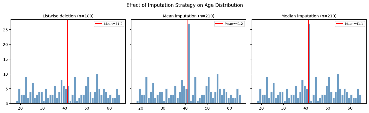

Mean imputation: creates a spike at the mean, suppresses variance.
Downstream covariance estimates will be biased downward.

5. Removing Duplicates¶

def deduplicate(arrays: list[np.ndarray]) -> list[np.ndarray]:
    """
    Remove rows where all features are identical.
    Returns deduplicated arrays and the boolean mask of kept rows.
    """
    # Stack into a matrix for row-wise comparison
    # Handle NaN by treating np.nan == np.nan as True (for dedup purposes)
    n_rows = len(arrays[0])
    seen   = set()
    keep   = np.ones(n_rows, dtype=bool)

    for i in range(n_rows):
        key = tuple(float(a[i]) if not isinstance(a[i], str) else a[i] for a in arrays)
        if key in seen:
            keep[i] = False
        else:
            seen.add(key)

    return [a[keep] for a in arrays], keep

arrays_clean, keep_mask = deduplicate([age_full, revenue_full, raw_country])
age_dedup, revenue_dedup, country_dedup = arrays_clean

print(f"Before dedup: {len(age_full)} rows")
print(f"After  dedup: {len(age_dedup)} rows")
print(f"Removed: {len(age_full) - len(age_dedup)} duplicates")

Before dedup: 210 rows
After  dedup: 203 rows
Removed: 7 duplicates

6. Detecting and Handling Outliers¶

An outlier is not automatically an error. It may be:

A measurement error → remove it
An extreme but valid observation → keep it, use robust statistics
A data entry error → correct it if possible

Two standard detection methods:

IQR rule: flag values below Q1 − 1.5·IQR or above Q3 + 1.5·IQR
Z-score rule: flag values with |z| > 3 (assumes near-normal distribution)

def flag_outliers_iqr(arr: np.ndarray, k: float = 1.5) -> np.ndarray:
    """Returns boolean mask: True where value is an outlier."""
    clean = arr[~np.isnan(arr)]
    q1, q3 = np.percentile(clean, [25, 75])
    iqr = q3 - q1
    return (arr < q1 - k * iqr) | (arr > q3 + k * iqr)

def flag_outliers_zscore(arr: np.ndarray, threshold: float = 3.0) -> np.ndarray:
    """Returns boolean mask: True where |z-score| > threshold."""
    mean = np.nanmean(arr)
    std  = np.nanstd(arr)
    z    = (arr - mean) / std
    return np.abs(z) > threshold

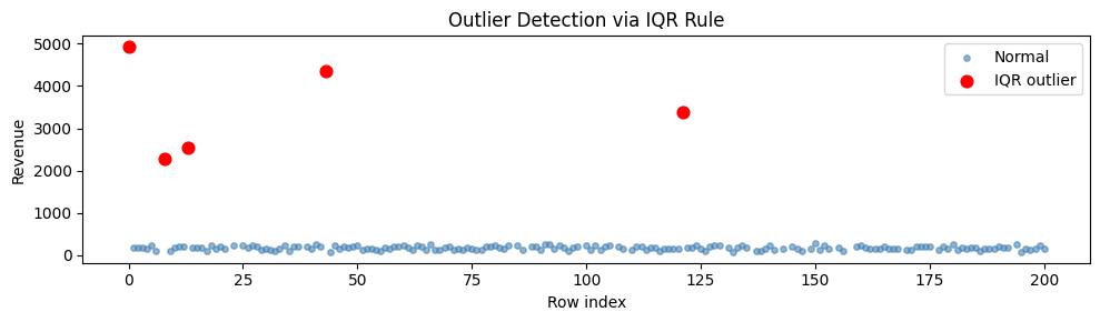
rev = revenue_dedup
iqr_mask    = flag_outliers_iqr(rev)
zscore_mask = flag_outliers_zscore(rev)

print(f"IQR rule flags    {iqr_mask.sum()} outliers")
print(f"Z-score rule flags {zscore_mask.sum()} outliers")

fig, ax = plt.subplots(figsize=(10, 3))
valid = ~np.isnan(rev)
ax.scatter(np.where(valid)[0], rev[valid], s=15, color='steelblue', alpha=0.6, label='Normal')
ax.scatter(np.where(iqr_mask)[0], rev[iqr_mask], s=60, color='red', zorder=5, label='IQR outlier')
ax.set_xlabel('Row index'); ax.set_ylabel('Revenue')
ax.set_title('Outlier Detection via IQR Rule')
ax.legend()
plt.tight_layout()
plt.show()

# Winsorize as an alternative to removal
def winsorize(arr: np.ndarray, lower: float = 1.0, upper: float = 99.0) -> np.ndarray:
    """Clip values at given percentiles."""
    lo, hi = np.nanpercentile(arr, [lower, upper])
    return np.clip(arr, lo, hi)

rev_winsorized = winsorize(rev)
print(f"\nBefore winsorize: max={np.nanmax(rev):.0f}, mean={np.nanmean(rev):.1f}")
print(f"After  winsorize: max={np.nanmax(rev_winsorized):.0f}, mean={np.nanmean(rev_winsorized):.1f}")

IQR rule flags    5 outliers
Z-score rule flags 5 outliers


Before winsorize: max=4940, mean=266.2
After  winsorize: max=3571, mean=254.5

7. Encoding Standardization¶

COUNTRY_MAP = {
    'us':            'US',
    'united states': 'US',
    'usa':           'US',
    'uk':            'UK',
    'united kingdom':'UK',
    'de':            'DE',
    'germany':       'DE',
    'fr':            'FR',
    'france':        'FR',
}

def standardize_country(arr: np.ndarray) -> np.ndarray:
    """Normalize country strings to canonical 2-letter codes."""
    result = np.empty_like(arr)
    for i, val in enumerate(arr):
        key = str(val).strip().lower()
        result[i] = COUNTRY_MAP.get(key, val.strip().upper())
    return result

country_clean = standardize_country(country_dedup)

raw_unique, raw_counts = np.unique(country_dedup, return_counts=True)
cln_unique, cln_counts = np.unique(country_clean, return_counts=True)

print("Before standardization:", dict(zip(raw_unique, raw_counts)))
print("After  standardization:", dict(zip(cln_unique, cln_counts)))

Before standardization: {np.str_(' D'): np.int64(5), np.str_('DE'): np.int64(53), np.str_('FR'): np.int64(48), np.str_('UK'): np.int64(43), np.str_('US'): np.int64(44), np.str_('Un'): np.int64(5), np.str_('us'): np.int64(5)}
After  standardization: {np.str_('D'): np.int64(5), np.str_('DE'): np.int64(53), np.str_('FR'): np.int64(48), np.str_('UK'): np.int64(43), np.str_('UN'): np.int64(5), np.str_('US'): np.int64(49)}

8. A Cleaning Pipeline¶

def clean_dataset(
    age_raw: np.ndarray,
    revenue_raw: np.ndarray,
    country_raw: np.ndarray,
) -> dict:
    """
    Full cleaning pipeline:
    1. Deduplicate
    2. Standardize encoding
    3. Flag and winsorize outliers
    4. Median-impute missing values
    Returns a dict of cleaned arrays and a cleaning report.
    """
    report = {}
    n0 = len(age_raw)

    # Step 1
    (age, revenue, country), _ = deduplicate([age_raw, revenue_raw, country_raw])
    report['duplicates_removed'] = n0 - len(age)

    # Step 2
    country = standardize_country(country)

    # Step 3
    revenue_iqr_outliers = flag_outliers_iqr(revenue).sum()
    revenue = winsorize(revenue)
    report['revenue_outliers_winsorized'] = int(revenue_iqr_outliers)

    # Step 4
    report['missing_age_imputed'] = int(np.isnan(age).sum())
    report['missing_revenue_imputed'] = int(np.isnan(revenue).sum())
    age     = impute_median(age)
    revenue = impute_median(revenue)

    report['final_n'] = len(age)
    return {'age': age, 'revenue': revenue, 'country': country}, report

cleaned, report = clean_dataset(age_full, revenue_full, raw_country)

print("=== Cleaning Report ===")
for k, v in report.items():
    print(f"  {k}: {v}")

print(f"\nFinal dataset: {report['final_n']} rows, 0 NaN")
print(f"NaN in age:    {np.isnan(cleaned['age']).sum()}")
print(f"NaN in revenue:{np.isnan(cleaned['revenue']).sum()}")

=== Cleaning Report ===
  duplicates_removed: 7
  revenue_outliers_winsorized: 5
  missing_age_imputed: 21
  missing_revenue_imputed: 22
  final_n: 203

Final dataset: 203 rows, 0 NaN
NaN in age:    0
NaN in revenue:0

9. What Comes Next¶

With a clean dataset, you can compute meaningful summaries. ch273 — Descriptive Statistics formalizes mean, median, variance, skewness, and their relationships. The outlier effects you observed in section 6 will reappear there quantitatively.

The imputation choices made here propagate through every downstream analysis. In ch276 — Bias and Variance, you will see that mean imputation specifically inflates the bias of covariance estimates — a concrete consequence of the design choice made in this chapter.