(Continues ch281 — Regression; connects to bias-variance from ch276)
1. Training Error Is Not Generalization Error
Any model can be made to fit its training data arbitrarily well by increasing complexity. The question that matters is: how well does it predict data it has never seen?
Generalization error = error on new, unseen data from the same distribution.
All evaluation must be done on data that was not used in training.
2. Regression Metrics
import numpy as np
import matplotlib.pyplot as plt
from scipy import stats

rng = np.random.default_rng(42)

def mse(y_true, y_pred):  return np.mean((y_true - y_pred)**2)
def rmse(y_true, y_pred): return np.sqrt(mse(y_true, y_pred))
def mae(y_true, y_pred):  return np.mean(np.abs(y_true - y_pred))
def r2(y_true, y_pred):
    ss_res = np.sum((y_true - y_pred)**2)
    ss_tot = np.sum((y_true - y_true.mean())**2)
    return 1 - ss_res / ss_tot
def mape(y_true, y_pred): return np.mean(np.abs((y_true - y_pred)/y_true)) * 100

# Generate dataset
n = 300
x = rng.normal(0, 1, n)
y_true = 2 + 3*x + rng.normal(0, 2, n)

# Three predictions: good, biased, noisy
predictions = {
    'Good':   2.1 + 2.9*x + rng.normal(0, 2.1, n),
    'Biased': 5.0 + 2.9*x + rng.normal(0, 2.0, n),  # intercept wrong
    'Noisy':  2.0 + 3.0*x + rng.normal(0, 6.0, n),  # high variance
}

print(f"{'Predictor':<12} {'MSE':>7} {'RMSE':>7} {'MAE':>7} {'R²':>7}")
print('-' * 48)
for name, y_pred in predictions.items():
    print(f"{name:<12} {mse(y_true,y_pred):>7.3f} {rmse(y_true,y_pred):>7.3f} "
          f"{mae(y_true,y_pred):>7.3f} {r2(y_true,y_pred):>7.3f}")
Predictor MSE RMSE MAE R²
------------------------------------------------
Good 9.851 3.139 2.542 0.196
Biased 18.481 4.299 3.569 -0.508
Noisy 43.781 6.617 5.244 -2.573
3. Classification Metrics
def confusion_matrix(y_true: np.ndarray, y_pred: np.ndarray) -> np.ndarray:
"""2x2 confusion matrix: [[TN, FP], [FN, TP]]."""
tn = np.sum((y_true == 0) & (y_pred == 0))
fp = np.sum((y_true == 0) & (y_pred == 1))
fn = np.sum((y_true == 1) & (y_pred == 0))
tp = np.sum((y_true == 1) & (y_pred == 1))
return np.array([[tn, fp], [fn, tp]])
def classification_report(y_true, y_pred):
cm = confusion_matrix(y_true, y_pred)
tn, fp, fn, tp = cm[0,0], cm[0,1], cm[1,0], cm[1,1]
accuracy = (tp + tn) / (tp + tn + fp + fn)
precision = tp / (tp + fp) if (tp + fp) > 0 else 0
recall = tp / (tp + fn) if (tp + fn) > 0 else 0
f1 = 2 * precision * recall / (precision + recall) if (precision + recall) > 0 else 0
return {'accuracy': accuracy, 'precision': precision, 'recall': recall, 'f1': f1, 'cm': cm}
def roc_auc(y_true: np.ndarray, y_score: np.ndarray) -> tuple[np.ndarray, np.ndarray, float]:
"""Returns (fpr, tpr, auc) for the ROC curve."""
thresholds = np.sort(np.unique(y_score))[::-1]
fpr_list, tpr_list = [0], [0]
n_pos = y_true.sum()
n_neg = len(y_true) - n_pos
for t in thresholds:
y_pred = (y_score >= t).astype(int)
r = classification_report(y_true, y_pred)
fpr_list.append(1 - r['accuracy'] * len(y_true) / n_neg - r['recall'] * n_pos/n_neg + 1)
# Use direct formula
cm = r['cm']
tpr_list.append(cm[1,1] / n_pos if n_pos > 0 else 0)
fpr_list[-1] = cm[0,1] / n_neg if n_neg > 0 else 0
fpr = np.array(fpr_list + [1])
tpr = np.array(tpr_list + [1])
auc = np.trapezoid(tpr, fpr)
return fpr, tpr, auc
# Generate binary classification data
n_cls = 400
x_cls = rng.normal(0, 1, (n_cls, 2))
y_cls = (x_cls[:, 0] + x_cls[:, 1] + rng.normal(0, 0.5, n_cls) > 0).astype(int)
# Simple logistic model: sigmoid of linear combination
def sigmoid(z): return 1 / (1 + np.exp(-z))
z_score = x_cls[:, 0] + x_cls[:, 1] + rng.normal(0, 0.3, n_cls)
y_prob = sigmoid(z_score)
y_pred_cls = (y_prob > 0.5).astype(int)
rep = classification_report(y_cls, y_pred_cls)
print("Classification Metrics:")
for k, v in rep.items():
if k != 'cm':
print(f" {k}: {v:.4f}")
print(f"\nConfusion matrix:\n{rep['cm']}")
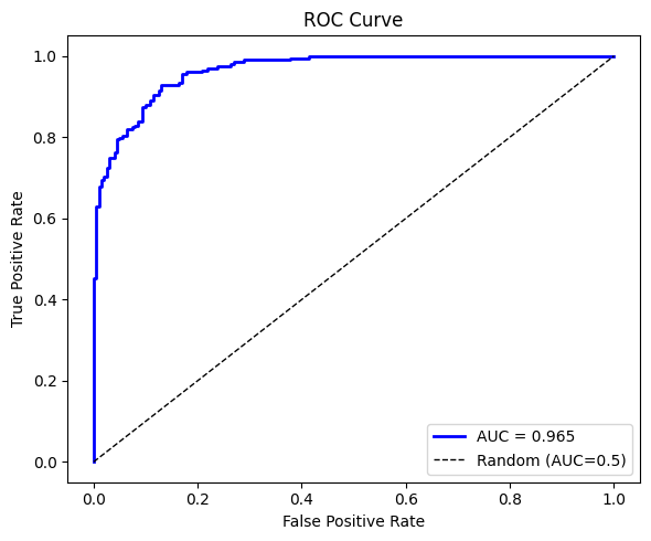
fpr, tpr, auc = roc_auc(y_cls, y_prob)
fig, ax = plt.subplots(figsize=(6, 5))
ax.plot(fpr, tpr, 'b-', lw=2, label=f'AUC = {auc:.3f}')
ax.plot([0,1],[0,1],'k--', lw=1, label='Random (AUC=0.5)')
ax.set_xlabel('False Positive Rate')
ax.set_ylabel('True Positive Rate')
ax.set_title('ROC Curve')
ax.legend()
plt.tight_layout()
plt.show()Classification Metrics:
accuracy: 0.8900
precision: 0.8856
recall: 0.8945
f1: 0.8900
Confusion matrix:
[[178 23]
[ 21 178]]
4. The Train/Test Split
def train_test_split(
    *arrays, test_size: float = 0.2, rng = None
):
    """Split arrays into random train and test subsets."""
    if rng is None: rng = np.random.default_rng()
    n   = len(arrays[0])
    idx = rng.permutation(n)
    n_test = int(n * test_size)
    test_idx  = idx[:n_test]
    train_idx = idx[n_test:]
    return tuple(a[train_idx] for a in arrays) + tuple(a[test_idx] for a in arrays)

n = 200
xr = rng.normal(0, 1, n)
yr = 2 + 3*xr + rng.normal(0, 2, n)

x_tr, y_tr, x_te, y_te = train_test_split(xr, yr, test_size=0.2, rng=rng)

def fit_and_eval(x_tr, y_tr, x_te, y_te, degree):
    b = np.polyfit(x_tr, y_tr, degree)
    return (
        mse(y_tr, np.polyval(b, x_tr)),
        mse(y_te, np.polyval(b, x_te))
    )

degrees = range(1, 15)
train_mses = []
test_mses  = []

for d in degrees:
    tr_mse, te_mse = fit_and_eval(x_tr, y_tr, x_te, y_te, d)
    train_mses.append(tr_mse)
    test_mses.append(te_mse)

fig, ax = plt.subplots(figsize=(9, 4))
ax.plot(degrees, train_mses, 'o-', color='blue',  label='Train MSE')
ax.plot(degrees, test_mses,  's-', color='red',   label='Test MSE')
ax.set_xlabel('Polynomial degree')
ax.set_ylabel('MSE')
ax.set_ylim(0, 30)
ax.set_title('Train vs Test MSE — the overfitting signature')
ax.legend()
plt.tight_layout()
plt.show()

print("Train MSE monotonically decreases. Test MSE has a minimum.")
print("The gap between them is the overfitting gap.")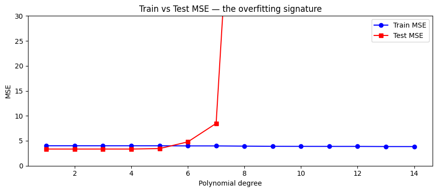
Train MSE monotonically decreases. Test MSE has a minimum.
The gap between them is the overfitting gap.
5. What Comes Next
The train/test gap just visualized is overfitting. ch283 — Overfitting explains it mechanically via the bias-variance tradeoff and presents regularization as a remedy. ch284 — Cross Validation replaces the single random train/test split with a procedure that gives a more stable estimate of generalization error.