(Synthesizes: gradient descent ch213, chain rule ch216, matrix multiply ch154, sigmoid ch063, softmax+cross-entropy ch294)
1. What a Neural Network Is Mathematically
A neural network is a composition of parametric functions:
Each layer applies an affine transformation followed by a non-linear activation:
Training finds that minimizes a loss function via gradient descent on the gradient computed by backpropagation.
2. Forward Pass
import numpy as np
import matplotlib.pyplot as plt
rng = np.random.default_rng(42)
def relu(z): return np.maximum(0, z)
def relu_grad(z): return (z > 0).astype(float)
def sigmoid(z):
return np.where(z >= 0, 1/(1+np.exp(-z)), np.exp(z)/(1+np.exp(z)))
def sigmoid_grad(z):
s = sigmoid(z)
return s * (1 - s)
def softmax(Z):
Z_s = Z - Z.max(axis=1, keepdims=True)
e = np.exp(Z_s)
return e / e.sum(axis=1, keepdims=True)
class NeuralNetworkFromScratch:
"""
Fully-connected neural network: [input -> hidden1 -> hidden2 -> output]
Trained with mini-batch SGD and backpropagation.
"""
def __init__(self, layer_sizes, lr=0.01, rng=None):
self.rng = rng or np.random.default_rng()
self.lr = lr
self.params = self._init_params(layer_sizes)
def _init_params(self, sizes):
# He initialization for ReLU layers
params = []
for i in range(len(sizes) - 1):
fan_in = sizes[i]
W = self.rng.normal(0, np.sqrt(2 / fan_in), (sizes[i], sizes[i+1]))
b = np.zeros(sizes[i+1])
params.append({'W': W, 'b': b})
return params
def forward(self, X):
"""Return list of (z, a) for each layer."""
cache = []
a = X
for i, p in enumerate(self.params[:-1]): # hidden layers: ReLU
z = a @ p['W'] + p['b']
a = relu(z)
cache.append({'z': z, 'a': a})
# Output layer: softmax
p = self.params[-1]
z = a @ p['W'] + p['b']
a = softmax(z)
cache.append({'z': z, 'a': a})
return cache
def loss(self, y_pred, y_true_onehot):
eps = 1e-15
return -np.mean(np.sum(y_true_onehot * np.log(np.clip(y_pred, eps, 1)), axis=1))
def backward(self, X, cache, y_true_onehot):
"""Backpropagation: compute gradients for all parameters."""
n = len(X)
grads = [None] * len(self.params)
# Output layer gradient: d(CE)/d(z_L) = softmax - y (for softmax + CE)
dz = cache[-1]['a'] - y_true_onehot # (n, K)
# Activation of previous layer (or input)
a_prev = cache[-2]['a'] if len(cache) > 1 else X
grads[-1] = {
'dW': a_prev.T @ dz / n,
'db': dz.mean(axis=0),
}
# Propagate backward through hidden layers
da = dz @ self.params[-1]['W'].T
for i in range(len(self.params) - 2, -1, -1):
dz = da * relu_grad(cache[i]['z'])
a_prev = cache[i-1]['a'] if i > 0 else X
grads[i] = {
'dW': a_prev.T @ dz / n,
'db': dz.mean(axis=0),
}
da = dz @ self.params[i]['W'].T
return grads
def update(self, grads):
for p, g in zip(self.params, grads):
p['W'] -= self.lr * g['dW']
p['b'] -= self.lr * g['db']
def fit(self, X, y_onehot, n_epochs=200, batch_size=64):
losses = []
n = len(X)
for epoch in range(n_epochs):
idx = self.rng.permutation(n)
epoch_loss = []
for start in range(0, n, batch_size):
batch = idx[start:start+batch_size]
Xb, yb = X[batch], y_onehot[batch]
cache = self.forward(Xb)
loss = self.loss(cache[-1]['a'], yb)
grads = self.backward(Xb, cache, yb)
self.update(grads)
epoch_loss.append(loss)
losses.append(np.mean(epoch_loss))
return losses
def predict(self, X):
return np.argmax(self.forward(X)[-1]['a'], axis=1)
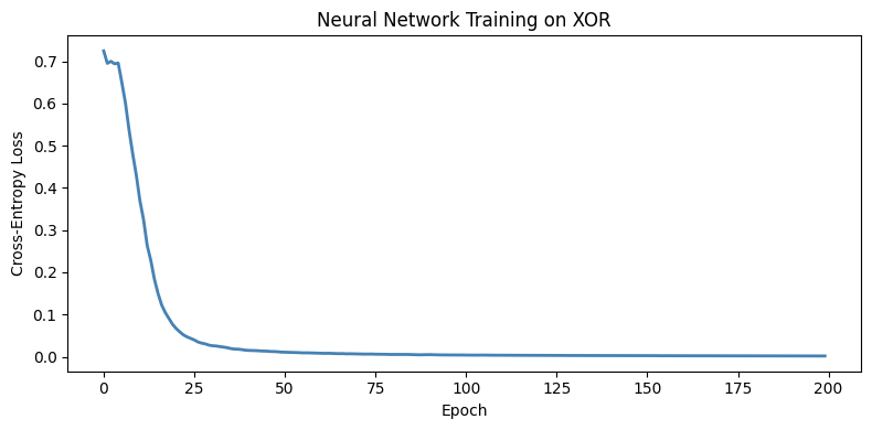
# Test on XOR (not linearly separable)
X_xor = np.array([[0,0],[0,1],[1,0],[1,1]], dtype=float)
y_xor = np.array([0, 1, 1, 0])
y_xor_oh = np.eye(2)[y_xor]
nn = NeuralNetworkFromScratch([2, 4, 2], lr=0.5, rng=rng)
losses = nn.fit(np.tile(X_xor, (100,1)), np.tile(y_xor_oh, (100,1)), n_epochs=200)
preds = nn.predict(X_xor)
print('XOR predictions:', preds, '| True:', y_xor)
print('Accuracy:', (preds == y_xor).mean())
fig, ax = plt.subplots(figsize=(8, 4))
ax.plot(losses, color='steelblue', lw=2)
ax.set_xlabel('Epoch'); ax.set_ylabel('Cross-Entropy Loss')
ax.set_title('Neural Network Training on XOR')
plt.tight_layout()
plt.show()XOR predictions: [0 1 1 0] | True: [0 1 1 0]
Accuracy: 1.0
3. Backpropagation as Chain Rule
Backpropagation is the chain rule (introduced in ch216) applied systematically through the computation graph.
For a network with loss , layer output :
The gradient flows backward through the network. Each layer computes its local gradient and multiplies by the upstream gradient.
# Visualize gradient magnitudes across layers during training
from sklearn.datasets import load_digits
from sklearn.preprocessing import OneHotEncoder
digits = load_digits()
X_d = digits.data / 16.0 # scale to [0,1]
y_d = digits.target
ohe = OneHotEncoder(sparse_output=False)
y_d_oh = ohe.fit_transform(y_d.reshape(-1, 1))
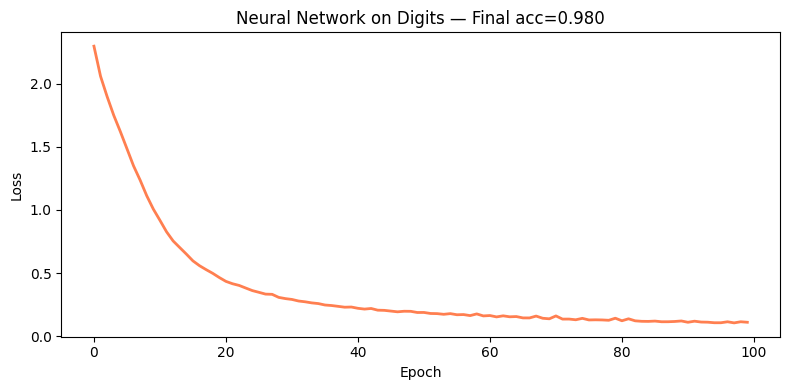
nn_digits = NeuralNetworkFromScratch([64, 128, 64, 10], lr=0.01, rng=rng)
losses_d = nn_digits.fit(X_d, y_d_oh, n_epochs=100, batch_size=64)
pred_d = nn_digits.predict(X_d)
acc_d = (pred_d == y_d).mean()
print(f'Digits accuracy (train): {acc_d:.4f}')
fig, ax = plt.subplots(figsize=(8, 4))
ax.plot(losses_d, color='coral', lw=2)
ax.set_xlabel('Epoch'); ax.set_ylabel('Loss')
ax.set_title(f'Neural Network on Digits — Final acc={acc_d:.3f}')
plt.tight_layout()
plt.show()Digits accuracy (train): 0.9800
4. What Comes Next
This neural network is trained with vanilla SGD. ch296 — Optimization Methods develops Adam, momentum, learning rate schedules, and weight decay — all the engineering that makes large networks trainable. The backpropagation algorithm implemented here is the core of every modern deep learning framework; the framework just builds the computation graph automatically.