ch301 — What is Deep Learning? - Mathematics for Programmers

1. The core claim¶

Deep learning is the practice of approximating functions by composing many simple, parameterised operations and adjusting parameters via gradient-guided optimisation.

That sentence is precise. Every word matters:

Approximating functions: we do not derive the mapping analytically; we search for it.
Composing: the power comes from depth — chaining simple transformations.
Parameterised: every operation has tunable numbers (weights, biases).
Gradient-guided: we use calculus (introduced in ch201) to know which direction to move.

2. Why depth?¶

The Universal Approximation Theorem (Cybenko, 1989; Hornik, 1991) states that a single hidden layer with enough neurons can approximate any continuous function on a compact domain. This sounds like depth is unnecessary.

It isn’t — for two reasons:

Width vs depth efficiency. Some functions require exponentially many neurons to represent with one layer, but only polynomially many across multiple layers.
Learning hierarchy. In practice, depth allows the network to learn reusable intermediate representations: edges → textures → shapes → objects (in vision), tokens → syntax → semantics (in language). Shallow networks cannot do this — they must learn everything at once.

3. The learning process as function search¶

Define:

$\mathcal{F}_\theta$ — a family of functions indexed by parameters $\theta \in \mathbb{R}^p$
$\mathcal{L}(\theta)$ — a loss function measuring how wrong $f_\theta$ is on training data
Training — finding $\theta^* = \arg\min_\theta \mathcal{L}(\theta)$ approximately, via gradient descent

This framing means every architectural choice is a statement about which function families you want to search over. CNNs search over translation-equivariant functions. Transformers search over functions with dynamic attention-weighted aggregation.

(Loss functions formalised in ch305; gradient descent mechanics in ch307.)

import numpy as np
import matplotlib.pyplot as plt

# Demonstrate: same task, very different function families
rng = np.random.default_rng(0)
x = np.linspace(-3, 3, 200)
y_true = np.sin(x) + 0.3 * np.cos(3 * x)  # true underlying function
x_obs = rng.uniform(-3, 3, 30)
y_obs = np.sin(x_obs) + 0.3 * np.cos(3 * x_obs) + rng.normal(0, 0.15, 30)

# Family 1: polynomials of varying degree
fig, axes = plt.subplots(1, 3, figsize=(14, 4))
degrees = [1, 4, 12]
titles = ['Degree-1 (linear)\nunderfits', 'Degree-4\ngood fit', 'Degree-12\noverfits']

for ax, deg, title in zip(axes, degrees, titles):
    coeffs = np.polyfit(x_obs, y_obs, deg)
    y_pred = np.polyval(coeffs, x)
    ax.plot(x, y_true, 'k--', lw=1.5, label='True function', alpha=0.6)
    ax.plot(x, y_pred, 'r-', lw=2, label=f'Degree-{deg} fit')
    ax.scatter(x_obs, y_obs, s=25, color='gray', zorder=3, alpha=0.8)
    ax.set_title(title)
    ax.set_ylim(-2.5, 2.5)
    ax.legend(fontsize=8)

plt.suptitle('Function families: choosing hypothesis class determines what you can learn',
             fontsize=12)
plt.tight_layout()
plt.savefig('ch301_function_families.png', dpi=120)
plt.show()

print("Key insight: The choice of family constrains what the learning algorithm can find.")
print("Neural networks define a very expressive family — but expressivity is not the same")
print("as learnability. Training dynamics matter as much as architecture.")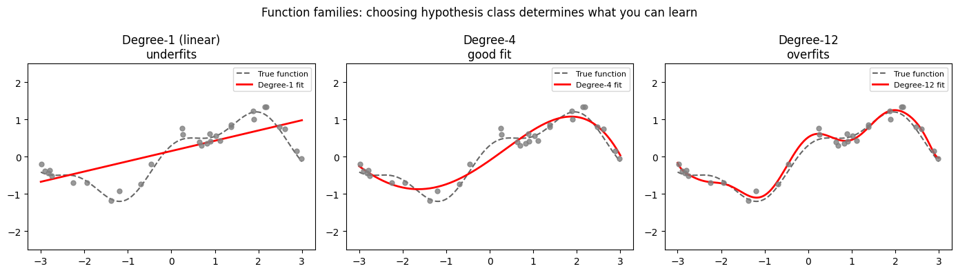

Key insight: The choice of family constrains what the learning algorithm can find.
Neural networks define a very expressive family — but expressivity is not the same
as learnability. Training dynamics matter as much as architecture.

4. A brief history in five inflection points¶

Year	Event	Why it mattered
1958	Rosenblatt perceptron	First trainable linear classifier
1986	Rumelhart et al. — backprop	Efficient gradient computation for MLPs
2012	AlexNet wins ImageNet by 10pp	Deep CNNs + GPUs + large data = new paradigm
2017	Attention is All You Need	Transformers replace RNNs for sequences
2020–	GPT-3 / scaling laws	Emergent capabilities at scale; LLMs as foundation models

Each inflection required the same three things simultaneously: better algorithms, more data, and faster hardware. None of the three alone was sufficient.

5. The supervised learning setup¶

Throughout Part X the default setting is supervised learning:

Training set: $\{(x^{(i)}, y^{(i)})\}_{i=1}^N$
Model: $\hat{y} = f_\theta(x)$
Loss: $\mathcal{L}(\theta) = \frac{1}{N} \sum_i \ell(\hat{y}^{(i)}, y^{(i)})$
Goal: $\theta^* \approx \arg\min_\theta \mathcal{L}(\theta)$

The subscript $\theta$ will always denote learnable parameters. $\ell$ is the per-sample loss (MSE for regression, cross-entropy for classification).

6. What deep learning is not¶

It is not magic. Every operation is differentiable arithmetic.
It is not guaranteed to find a global minimum. It finds good local minima.
It is not a replacement for understanding the problem. Architecture choices encode inductive biases.
It is not data-agnostic. The distribution of training data determines what generalises.

7. Notation used throughout Part X¶

Symbol	Meaning
$L$	Number of layers
$n_l$	Width of layer $l$
$W^{[l]}$	Weight matrix of layer $l$ , shape $(n_l, n_{l-1})$
$b^{[l]}$	Bias vector of layer $l$ , shape $(n_l,)$
$a^{[l]}$	Activation of layer $l$
$z^{[l]}$	Pre-activation: $W^{[l]} a^{[l-1]} + b^{[l]}$
$\sigma$	Activation function (context-dependent)
$\mathcal{L}$	Scalar loss
$\nabla_\theta \mathcal{L}$	Gradient of loss with respect to $\theta$

8. Summary¶

Deep learning = parameterised function composition + gradient-based optimisation.
Depth enables hierarchy of representations; this is why depth beats width in practice.
Every architectural choice is a hypothesis about the structure of the problem.
The mathematics is entirely the mathematics of Parts I–IX, applied at scale.

9. Forward and backward references¶

Used here: function composition (ch054), gradient descent (ch212), loss and residuals (ch072), activation functions (ch064–065), partial derivatives (ch210).

This will reappear in ch306 — Backpropagation from Scratch, where the abstract gradient computation described here becomes an explicit algorithm operating on the layer notation introduced in Section 7.