ch302 — The Perceptron - Mathematics for Programmers

1. What the perceptron computes¶

The perceptron is the atomic unit of neural computation. It takes a vector of inputs, computes a weighted sum, and passes the result through a threshold function:

\hat{y} = \mathbf{1}[\mathbf{w}^\top \mathbf{x} + b > 0]

(1)

where $\mathbf{w} \in \mathbb{R}^d$ are weights, $b \in \mathbb{R}$ is the bias, and $\mathbf{1}[\cdot]$ is the indicator function.

The geometric interpretation is immediate: $\mathbf{w}^\top \mathbf{x} + b = 0$ defines a hyperplane in $\mathbb{R}^d$ . The perceptron assigns class 1 to everything on one side, class 0 to the other. It is a linear classifier.

(Dot product geometry introduced in ch131–ch132. Hyperplanes are the generalisation of lines and planes from ch099–ch101.)

import numpy as np
import matplotlib.pyplot as plt
import matplotlib.patches as mpatches


class Perceptron:
    """Binary perceptron with the original Rosenblatt update rule."""

    def __init__(self, n_features: int, lr: float = 1.0, seed: int = 0):
        rng = np.random.default_rng(seed)
        self.w = rng.normal(0, 0.01, n_features)
        self.b = 0.0
        self.lr = lr

    def predict(self, X: np.ndarray) -> np.ndarray:
        """Return 0/1 predictions for each row of X."""
        return (X @ self.w + self.b > 0).astype(int)

    def fit(self, X: np.ndarray, y: np.ndarray, n_epochs: int = 20) -> list:
        """Train using the perceptron update rule. Returns per-epoch error counts."""
        errors_per_epoch = []
        for _ in range(n_epochs):
            errors = 0
            for xi, yi in zip(X, y):
                y_hat = int(xi @ self.w + self.b > 0)
                if y_hat != yi:
                    # Perceptron update: move decision boundary toward correct side
                    self.w += self.lr * (yi - y_hat) * xi
                    self.b += self.lr * (yi - y_hat)
                    errors += 1
            errors_per_epoch.append(errors)
        return errors_per_epoch


# --- Linearly separable dataset ---
rng = np.random.default_rng(7)
n = 60
X0 = rng.multivariate_normal([-1.5, -1.5], [[0.4, 0], [0, 0.4]], n // 2)
X1 = rng.multivariate_normal([1.5, 1.5], [[0.4, 0], [0, 0.4]], n // 2)
X = np.vstack([X0, X1])
y = np.array([0] * (n // 2) + [1] * (n // 2))

perc = Perceptron(n_features=2, lr=1.0)
errors = perc.fit(X, y, n_epochs=30)

# --- Plot: decision boundary + convergence ---
fig, (ax1, ax2) = plt.subplots(1, 2, figsize=(12, 5))

xx = np.linspace(-4, 4, 300)
# w[0]*x + w[1]*y + b = 0  =>  y = -(w[0]*x + b) / w[1]
if abs(perc.w[1]) > 1e-8:
    yy = -(perc.w[0] * xx + perc.b) / perc.w[1]
    ax1.plot(xx, yy, 'k-', lw=2, label='Decision boundary')

colors = ['#e74c3c', '#3498db']
for cls in [0, 1]:
    mask = y == cls
    ax1.scatter(X[mask, 0], X[mask, 1], color=colors[cls], s=40,
                alpha=0.8, label=f'Class {cls}', zorder=3)

ax1.set_xlim(-4, 4)
ax1.set_ylim(-4, 4)
ax1.set_aspect('equal')
ax1.set_title('Perceptron — learned decision boundary')
ax1.legend()
acc = (perc.predict(X) == y).mean()
ax1.set_xlabel(f'Final accuracy: {acc:.1%}')

ax2.plot(errors, 'o-', color='#2c3e50')
ax2.set_xlabel('Epoch')
ax2.set_ylabel('Misclassified samples')
ax2.set_title('Convergence (errors → 0 for separable data)')
ax2.axhline(0, color='green', linestyle='--', alpha=0.5)

plt.tight_layout()
plt.savefig('ch302_perceptron.png', dpi=120)
plt.show()
print(f"Converged in {errors.index(0) + 1 if 0 in errors else '>30'} epochs")
print(f"Learned weights: w={perc.w}, b={perc.b:.4f}")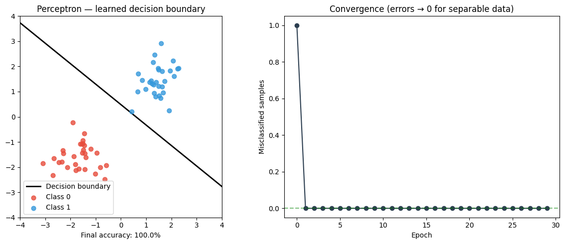

Converged in 2 epochs
Learned weights: w=[1.67463731 2.06193869], b=-1.0000

2. The perceptron update rule — why it works¶

When sample $(x, y)$ is misclassified:

\mathbf{w} \leftarrow \mathbf{w} + \eta (y - \hat{y}) \mathbf{x}, \quad b \leftarrow b + \eta (y - \hat{y})

(2)

For a false negative ( $y=1, \hat{y}=0$ ): we add $\mathbf{x}$ to $\mathbf{w}$ , making $\mathbf{w}^\top \mathbf{x}$ larger, pushing the prediction toward 1.

For a false positive ( $y=0, \hat{y}=1$ ): we subtract $\mathbf{x}$ from $\mathbf{w}$ .

Perceptron Convergence Theorem: If the data is linearly separable, the perceptron converges in finite steps. If not, it never converges — it cycles. This is the fundamental limitation that XOR famously exposed.

3. The XOR failure¶

# XOR: no linear boundary exists
X_xor = np.array([[0, 0], [0, 1], [1, 0], [1, 1]], dtype=float)
y_xor = np.array([0, 1, 1, 0])  # XOR labels

perc_xor = Perceptron(n_features=2, lr=1.0, seed=3)
errors_xor = perc_xor.fit(X_xor, y_xor, n_epochs=50)

fig, (ax1, ax2) = plt.subplots(1, 2, figsize=(11, 4))

markers = ['o', 's']
for i, (xi, yi) in enumerate(zip(X_xor, y_xor)):
    ax1.scatter(xi[0], xi[1], color=colors[yi], s=200, marker=markers[yi],
                zorder=5, edgecolors='black', linewidths=1.5)
    ax1.annotate(f'  XOR={yi}', xi, fontsize=10)

xx = np.linspace(-0.5, 1.5, 200)
if abs(perc_xor.w[1]) > 1e-8:
    yy = -(perc_xor.w[0] * xx + perc_xor.b) / perc_xor.w[1]
    ax1.plot(xx, yy, 'k--', lw=2, label='Best linear attempt')
ax1.set_xlim(-0.5, 1.5)
ax1.set_ylim(-0.5, 1.5)
ax1.set_title('XOR is not linearly separable\n(perceptron cannot solve it)')
ax1.legend()

ax2.plot(errors_xor, color='#c0392b')
ax2.set_title('Perceptron on XOR — never converges')
ax2.set_xlabel('Epoch')
ax2.set_ylabel('Errors')
ax2.set_ylim(0, 5)

plt.tight_layout()
plt.savefig('ch302_xor_failure.png', dpi=120)
plt.show()
print("Final accuracy on XOR:", (perc_xor.predict(X_xor) == y_xor).mean())
print("\nThe fix: stack perceptrons into layers — covered in ch303.")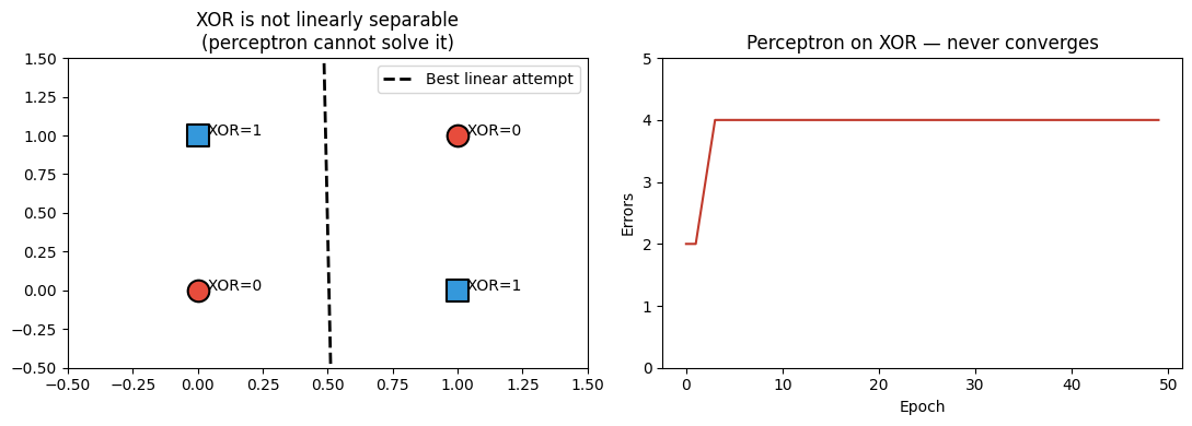

Final accuracy on XOR: 0.5

The fix: stack perceptrons into layers — covered in ch303.

4. From perceptron to neuron¶

The modern usage replaces the hard threshold $\mathbf{1}[z > 0]$ with a smooth activation function $\sigma(z)$ . This is critical: the hard threshold has zero gradient almost everywhere, making gradient-based training impossible.

\text{Perceptron:} \quad \hat{y} = \mathbf{1}[\mathbf{w}^\top\mathbf{x} + b > 0]

(3)

\text{Neuron:} \quad \hat{y} = \sigma(\mathbf{w}^\top\mathbf{x} + b)

(4)

Activation functions are explored in depth in ch309. The chain rule that enables gradient computation through $\sigma$ is formalised in ch306.

5. Summary¶

The perceptron computes a weighted sum then applies a threshold — it is a linear classifier.
The update rule moves the decision boundary toward the misclassified point.
The Perceptron Convergence Theorem guarantees convergence iff data is linearly separable.
XOR is the canonical failure: it requires a nonlinear boundary, forcing us toward multilayer nets.

6. Forward and backward references¶

Used here: dot product (ch131), hyperplanes from linear algebra (ch161), linear classifiers (ch287).

This will reappear in ch303 — Multilayer Networks, where stacking two perceptron-like layers solves XOR, and in ch306 — Backpropagation, where the hard threshold is replaced by a differentiable activation to enable learning.