ch305 — Loss Functions - Mathematics for Programmers

1. What a loss function is¶

A loss function $\ell(\hat{y}, y)$ measures the cost of predicting $\hat{y}$ when the true label is $y$ . The training loss is its average over the dataset:

\mathcal{L}(\theta) = \frac{1}{N} \sum_{i=1}^N \ell(f_\theta(x^{(i)}), y^{(i)})

(1)

Loss function design is not arbitrary. A good loss must:

Be differentiable almost everywhere (gradient descent requires $\nabla_\theta \mathcal{L}$ ).
Have a minimum at the correct prediction (otherwise the gradient points in the wrong direction).
Produce informative gradients even for nearly-correct predictions.
Be statistically principled — ideally derived from maximum likelihood estimation.

2. Mean Squared Error (regression)¶

\ell_{\text{MSE}}(\hat{y}, y) = (\hat{y} - y)^2

(2)

Gradient: $\partial \ell / \partial \hat{y} = 2(\hat{y} - y)$ . Linear in the residual — large errors produce large gradients, small errors produce small gradients.

Statistical derivation: MSE is the negative log-likelihood under a Gaussian noise model: $y \sim \mathcal{N}(f_\theta(x), \sigma^2)$ . Minimising MSE = maximising likelihood.

(Gaussian distribution: ch253. Log-likelihood: ch293.)

3. Binary Cross-Entropy (binary classification)¶

\ell_{\text{BCE}}(\hat{p}, y) = -[y \log \hat{p} + (1-y) \log(1-\hat{p})]

(3)

where $\hat{p} = \sigma(z) \in (0,1)$ is the predicted probability and $y \in \{0,1\}$ .

Why not MSE for classification? If the output is a probability from a sigmoid, MSE gradient $\frac{\partial \mathcal{L}}{\partial z} = (\hat{p} - y) \cdot \hat{p}(1-\hat{p})$ nearly vanishes when $\hat{p}$ is confident but wrong (sigmoid saturated). BCE gradient: $\frac{\partial \mathcal{L}}{\partial z} = \hat{p} - y$ — clean, non-vanishing.

(Entropy and KL divergence: ch294–ch295. Sigmoid: ch064.)

4. Categorical Cross-Entropy (multiclass)¶

\ell_{\text{CE}}(\hat{\mathbf{p}}, y) = -\log \hat{p}_y = -\sum_{k=1}^K y_k \log \hat{p}_k

(4)

where $\hat{\mathbf{p}} = \text{softmax}(\mathbf{z})$ and $y$ is one-hot encoded.

Softmax:

\hat{p}_k = \frac{e^{z_k}}{\sum_j e^{z_j}}

(5)

Combined gradient of CE + softmax: $\frac{\partial \mathcal{L}}{\partial \mathbf{z}} = \hat{\mathbf{p}} - \mathbf{y}$ . This elegant result is why CE+softmax is the universal choice for classification.

import numpy as np
import matplotlib.pyplot as plt


def mse(y_hat: np.ndarray, y: np.ndarray) -> float:
    return float(np.mean((y_hat - y) ** 2))


def bce(p_hat: np.ndarray, y: np.ndarray, eps: float = 1e-12) -> float:
    """Binary cross-entropy. Clips to avoid log(0)."""
    p = np.clip(p_hat, eps, 1 - eps)
    return float(-np.mean(y * np.log(p) + (1 - y) * np.log(1 - p)))


def softmax(z: np.ndarray) -> np.ndarray:
    """Numerically stable softmax using log-sum-exp trick."""
    z_shifted = z - z.max(axis=0, keepdims=True)
    exp_z = np.exp(z_shifted)
    return exp_z / exp_z.sum(axis=0, keepdims=True)


def cross_entropy(logits: np.ndarray, y_onehot: np.ndarray, eps: float = 1e-12) -> float:
    """Categorical cross-entropy from logits."""
    p = softmax(logits)
    return float(-np.mean(np.sum(y_onehot * np.log(p + eps), axis=0)))


# --- Visualise BCE vs MSE gradient behaviour ---
p = np.linspace(0.01, 0.99, 300)

# True label y=1
bce_loss = -(1 * np.log(p) + 0 * np.log(1 - p))
mse_loss = (1 - p) ** 2

# Gradients w.r.t. z (pre-sigmoid), using chain rule
# d(sigmoid)/dz = p*(1-p)
dbce_dz = p - 1          # p - y (when y=1)
dmse_dz = 2 * (p - 1) * p * (1 - p)   # MSE grad × sigmoid derivative

fig, axes = plt.subplots(2, 2, figsize=(12, 8))

for ax, loss, name, color in [
    (axes[0, 0], bce_loss, 'Binary Cross-Entropy (y=1)', '#e74c3c'),
    (axes[0, 1], mse_loss, 'MSE (y=1)', '#3498db'),
]:
    ax.plot(p, loss, color=color, lw=2)
    ax.set_xlabel('Predicted probability $\\hat{p}$')
    ax.set_ylabel('Loss')
    ax.set_title(name)
    ax.axvline(1.0, color='green', linestyle='--', alpha=0.5, label='Correct (p=1)')
    ax.legend()

for ax, grad, name, color in [
    (axes[1, 0], dbce_dz, 'BCE gradient w.r.t. z', '#e74c3c'),
    (axes[1, 1], dmse_dz, 'MSE gradient w.r.t. z', '#3498db'),
]:
    ax.plot(p, grad, color=color, lw=2)
    ax.axhline(0, color='black', alpha=0.3)
    ax.set_xlabel('Predicted probability $\\hat{p}$')
    ax.set_ylabel('Gradient')
    ax.set_title(name)
    ax.fill_between(p, grad, 0, alpha=0.15, color=color)

plt.suptitle('BCE has informative gradients even at extreme predictions;\n'
             'MSE gradient vanishes at saturation.', fontsize=11)
plt.tight_layout()
plt.savefig('ch305_loss_gradients.png', dpi=120)
plt.show()

# Demonstration: gradient magnitude at nearly-wrong confident prediction
p_wrong = 0.99  # predicted 0.99 but true label is 0
bce_grad = p_wrong - 0
mse_grad = 2 * (p_wrong - 0) * p_wrong * (1 - p_wrong)
print(f"Confident wrong prediction (p={p_wrong}, y=0):")
print(f"  BCE gradient |dL/dz| = {abs(bce_grad):.4f}  ← still strong")
print(f"  MSE gradient |dL/dz| = {abs(mse_grad):.4f}  ← nearly zero!")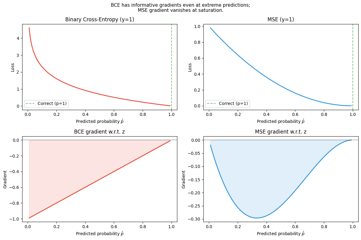

Confident wrong prediction (p=0.99, y=0):
  BCE gradient |dL/dz| = 0.9900  ← still strong
  MSE gradient |dL/dz| = 0.0196  ← nearly zero!

# --- Softmax behaviour ---
logits = np.array([[2.0, 1.0, 0.1, -1.0],
                   [5.0, 1.0, 0.1, -1.0],
                   [50.0, 1.0, 0.1, -1.0]])

print("Softmax concentrates probability mass as the winning logit grows:")
for z in logits:
    p = softmax(z[:, None]).ravel()
    print(f"  logits={z} → p={np.round(p, 3)}")

# Numerically UNSTABLE version for comparison
def softmax_unstable(z):
    exp_z = np.exp(z)
    return exp_z / exp_z.sum()

large_z = np.array([1000.0, 999.0, 998.0])
print(f"\nUnstable softmax on large logits: {softmax_unstable.__name__}")
try:
    result = softmax_unstable(large_z)
    print(f"  Result: {result}  (overflow produces NaN/inf if not handled)")
except Exception as e:
    print(f"  Exception: {e}")

stable_result = softmax(large_z[:, None]).ravel()
print(f"Stable softmax (log-sum-exp): {stable_result}")

Softmax concentrates probability mass as the winning logit grows:
  logits=[ 2.   1.   0.1 -1. ] → p=[0.638 0.235 0.095 0.032]
  logits=[ 5.   1.   0.1 -1. ] → p=[0.973 0.018 0.007 0.002]
  logits=[50.   1.   0.1 -1. ] → p=[1. 0. 0. 0.]

Unstable softmax on large logits: softmax_unstable
  Result: [nan nan nan]  (overflow produces NaN/inf if not handled)
Stable softmax (log-sum-exp): [0.66524096 0.24472847 0.09003057]

C:\Users\user\AppData\Local\Temp\ipykernel_25912\3083791601.py:13: RuntimeWarning: overflow encountered in exp
  exp_z = np.exp(z)
C:\Users\user\AppData\Local\Temp\ipykernel_25912\3083791601.py:14: RuntimeWarning: invalid value encountered in divide
  return exp_z / exp_z.sum()

5. Huber loss (robust regression)¶

MSE is sensitive to outliers because $(\hat{y} - y)^2$ grows quadratically. Huber loss interpolates between MSE (for small errors) and MAE (for large errors):

\ell_\delta(\hat{y}, y) = \begin{cases} \frac{1}{2}(\hat{y}-y)^2 & \text{if } |\hat{y}-y| \leq \delta \\ \delta\left(|\hat{y}-y| - \frac{\delta}{2}\right) & \text{otherwise} \end{cases}

(6)

Differentiable everywhere; gradient bounded by $\delta$ . Used in reinforcement learning (ch329) where reward estimates have heavy-tailed noise.

6. Choosing the loss function¶

Task	Output activation	Loss
Regression	Linear	MSE
Robust regression	Linear	Huber
Binary classification	Sigmoid	BCE
Multiclass (mutually exclusive)	Softmax	Categorical CE
Multilabel classification	Sigmoid (per class)	BCE (per class)
Generative models	Varies	KL divergence, ELBO

7. Summary¶

Loss functions must be differentiable and have informative gradients.
MSE = negative log-likelihood under Gaussian noise. BCE = negative log-likelihood for Bernoulli.
The BCE+sigmoid and CE+softmax gradients simplify to $\hat{p} - y$ — elegant and non-vanishing.
Loss choice encodes assumptions about the noise distribution of the labels.

8. Forward and backward references¶

Used here: entropy (ch294), KL divergence (ch295), Gaussian distribution (ch253), log-likelihood (ch293), sigmoid (ch064), derivatives (ch205–ch206).

This will reappear in ch306 — Backpropagation from Scratch, where the loss gradient $\partial \mathcal{L}/\partial \hat{y}$ is the starting point of the backward pass, and in ch325 — VAE, where the ELBO loss combines reconstruction CE and KL divergence.