ch306 — Backpropagation from Scratch - Mathematics for Programmers

1. The problem backprop solves¶

After the forward pass (ch304) we have a scalar loss $\mathcal{L}$ . We need $\frac{\partial \mathcal{L}}{\partial W^{[l]}}$ and $\frac{\partial \mathcal{L}}{\partial b^{[l]}}$ for every layer $l$ , so that gradient descent (ch307) can update the parameters.

Naively differentiating through a 50-layer network by hand is infeasible. Backpropagation (Rumelhart, Hinton, Williams, 1986) is the efficient algorithm for this: it applies the chain rule (ch215) in reverse topological order through the computation graph, reusing intermediate results so each gradient is computed exactly once.

Cost: one backward pass ≈ 2–3× the cost of one forward pass. Compare to finite differences: $O(p)$ forward passes for $p$ parameters — completely infeasible for millions of parameters.

2. Deriving the equations¶

Define the upstream gradient at layer $l$ as:

dA^{[l]} = \frac{\partial \mathcal{L}}{\partial A^{[l]}}

(1)

Working backwards from the loss:

Step 1 — Activation backward:

dZ^{[l]} = dA^{[l]} \odot \sigma'^{[l]}(Z^{[l]})

(2)

where $\odot$ is elementwise multiplication and $\sigma'$ is the derivative of the activation.

Step 2 — Linear backward:

dW^{[l]} = \frac{1}{B} \, dZ^{[l]} (A^{[l-1]})^\top

(3)

db^{[l]} = \frac{1}{B} \sum_{\text{batch}} dZ^{[l]}

(4)

dA^{[l-1]} = (W^{[l]})^\top dZ^{[l]}

(5)

The last equation propagates the gradient to the previous layer. Repeat for $l = L, L-1, \ldots, 1$ .

(Chain rule: ch215. Matrix transpose: ch154. Partial derivatives: ch210.)

import numpy as np


# ─────────────────────────────────────────────────────────────
# Activation functions and their exact derivatives
# ─────────────────────────────────────────────────────────────

def sigmoid(z):
    return 1.0 / (1.0 + np.exp(-np.clip(z, -500, 500)))

def sigmoid_grad(z):
    s = sigmoid(z)
    return s * (1.0 - s)

def relu(z):
    return np.maximum(0.0, z)

def relu_grad(z):
    return (z > 0).astype(float)

def softmax(z):
    z_s = z - z.max(axis=0, keepdims=True)
    e = np.exp(z_s)
    return e / e.sum(axis=0, keepdims=True)


# ─────────────────────────────────────────────────────────────
# Full MLP with forward + backward
# ─────────────────────────────────────────────────────────────

class MLPNumPy:
    """
    Feedforward network implemented entirely in NumPy.
    Supports arbitrary depth; last layer uses sigmoid for binary classification.
    Hidden layers use ReLU.
    """

    def __init__(self, layer_sizes: list, seed: int = 0):
        rng = np.random.default_rng(seed)
        self.params = {}
        self.n_layers = len(layer_sizes) - 1
        for l in range(1, len(layer_sizes)):
            fan_in = layer_sizes[l - 1]
            fan_out = layer_sizes[l]
            self.params[f'W{l}'] = rng.normal(0, np.sqrt(2.0 / fan_in), (fan_out, fan_in))
            self.params[f'b{l}'] = np.zeros(fan_out)

    def forward(self, X: np.ndarray) -> tuple:
        """
        X: shape (n_features, batch_size)
        Returns (output, cache)
        """
        cache = {'A0': X}
        A = X
        for l in range(1, self.n_layers + 1):
            W = self.params[f'W{l}']
            b = self.params[f'b{l}'][:, None]
            Z = W @ A + b
            cache[f'Z{l}'] = Z
            # Last layer: sigmoid; hidden layers: relu
            A = sigmoid(Z) if l == self.n_layers else relu(Z)
            cache[f'A{l}'] = A
        return A, cache

    def bce_loss(self, output: np.ndarray, y: np.ndarray) -> float:
        eps = 1e-12
        p = np.clip(output, eps, 1 - eps)
        return float(-np.mean(y * np.log(p) + (1 - y) * np.log(1 - p)))

    def backward(self, y: np.ndarray, cache: dict) -> dict:
        """
        y: shape (1, batch_size)
        Returns dict of gradients for all parameters.
        """
        grads = {}
        B = y.shape[1]
        L = self.n_layers

        # ── Gradient at output layer (BCE + sigmoid: dL/dZ = p - y) ──
        dA = cache[f'A{L}'] - y

        for l in range(L, 0, -1):
            A_prev = cache[f'A{l-1}']
            Z = cache[f'Z{l}']

            if l == L:
                # BCE + sigmoid: gradient already computed as dA = p - y
                dZ = dA
            else:
                # For hidden ReLU layers: dZ = dA * relu'(Z)
                dZ = dA * relu_grad(Z)

            grads[f'dW{l}'] = (dZ @ A_prev.T) / B
            grads[f'db{l}'] = dZ.mean(axis=1)
            dA = self.params[f'W{l}'].T @ dZ   # propagate to previous layer

        return grads

    def update(self, grads: dict, lr: float = 0.01):
        for l in range(1, self.n_layers + 1):
            self.params[f'W{l}'] -= lr * grads[f'dW{l}']
            self.params[f'b{l}'] -= lr * grads[f'db{l}']


# ─────────────────────────────────────────────────────────────
# Gradient check: numerical vs analytical
# ─────────────────────────────────────────────────────────────

def numerical_gradient(net, X, y, param_key, eps=1e-5):
    """Central-difference numerical gradient for one parameter matrix."""
    P = net.params[param_key]
    grad = np.zeros_like(P)
    for idx in np.ndindex(*P.shape):
        P[idx] += eps
        out_plus, _ = net.forward(X)
        loss_plus = net.bce_loss(out_plus, y)
        P[idx] -= 2 * eps
        out_minus, _ = net.forward(X)
        loss_minus = net.bce_loss(out_minus, y)
        P[idx] += eps
        grad[idx] = (loss_plus - loss_minus) / (2 * eps)
    return grad


rng = np.random.default_rng(7)
net = MLPNumPy([4, 6, 3, 1], seed=42)
X_test = rng.normal(0, 1, (4, 8))
y_test = rng.integers(0, 2, (1, 8)).astype(float)

out, cache = net.forward(X_test)
grads = net.backward(y_test, cache)

print("Gradient check (analytical vs numerical):")
print(f"{'Layer':<12} {'Max abs error':>15} {'Relative error':>16} {'Status':>10}")
print("-" * 56)

for l in range(1, net.n_layers + 1):
    key = f'W{l}'
    # Only check small matrices for speed
    if net.params[key].size > 50:
        print(f"  Layer {l} W: skipping (too large for numerical check)")
        continue
    num_grad = numerical_gradient(net, X_test, y_test, key)
    ana_grad = grads[f'd{key}']
    abs_err = np.max(np.abs(num_grad - ana_grad))
    rel_err = abs_err / (np.max(np.abs(num_grad)) + 1e-10)
    status = '✓ PASS' if rel_err < 1e-4 else '✗ FAIL'
    print(f"  Layer {l} W:  {abs_err:>15.2e}  {rel_err:>16.2e}  {status:>10}")

print("\nNumerical gradient check confirms analytical backprop is correct.")

Gradient check (analytical vs numerical):
Layer          Max abs error   Relative error     Status
--------------------------------------------------------
  Layer 1 W:         6.44e-12          2.81e-10      ✓ PASS
  Layer 2 W:         6.51e-12          2.20e-10      ✓ PASS
  Layer 3 W:         2.42e-12          9.23e-11      ✓ PASS

Numerical gradient check confirms analytical backprop is correct.

import matplotlib.pyplot as plt

# Train on a small dataset to verify the full loop works
rng = np.random.default_rng(0)
n = 200
X0 = rng.multivariate_normal([-1, -1], [[0.5, 0], [0, 0.5]], n // 2)
X1 = rng.multivariate_normal([1, 1], [[0.5, 0], [0, 0.5]], n // 2)
X_tr = np.vstack([X0, X1]).T  # shape (2, 200)
y_tr = np.array([0] * (n // 2) + [1] * (n // 2), dtype=float)[None, :]  # shape (1, 200)

net2 = MLPNumPy([2, 8, 8, 1], seed=1)
lr = 0.1
losses = []

for epoch in range(300):
    out, cache = net2.forward(X_tr)
    loss = net2.bce_loss(out, y_tr)
    losses.append(loss)
    grads = net2.backward(y_tr, cache)
    net2.update(grads, lr=lr)

preds = (net2.forward(X_tr)[0] > 0.5).astype(int)
acc = (preds == y_tr).mean()

fig, (ax1, ax2) = plt.subplots(1, 2, figsize=(12, 4))

ax1.plot(losses, color='#e74c3c', lw=2)
ax1.set_title('Training loss (BCE) vs epoch')
ax1.set_xlabel('Epoch')
ax1.set_ylabel('Loss')

# Decision boundary
xx, yy = np.meshgrid(np.linspace(-3, 3, 200), np.linspace(-3, 3, 200))
grid = np.c_[xx.ravel(), yy.ravel()].T
Z = net2.forward(grid)[0].reshape(xx.shape)
ax2.contourf(xx, yy, Z, levels=50, cmap='RdBu_r', alpha=0.7)
ax2.contour(xx, yy, Z, levels=[0.5], colors='k', linewidths=2)
colors = ['#e74c3c', '#3498db']
for cls in [0, 1]:
    mask = (y_tr.ravel() == cls)
    ax2.scatter(X_tr[0, mask], X_tr[1, mask], color=colors[cls], s=20, alpha=0.7)
ax2.set_title(f'Learned boundary (accuracy: {acc:.1%})')
ax2.set_aspect('equal')

plt.tight_layout()
plt.savefig('ch306_backprop.png', dpi=120)
plt.show()
print(f"Final loss: {losses[-1]:.4f} | Accuracy: {acc:.1%}")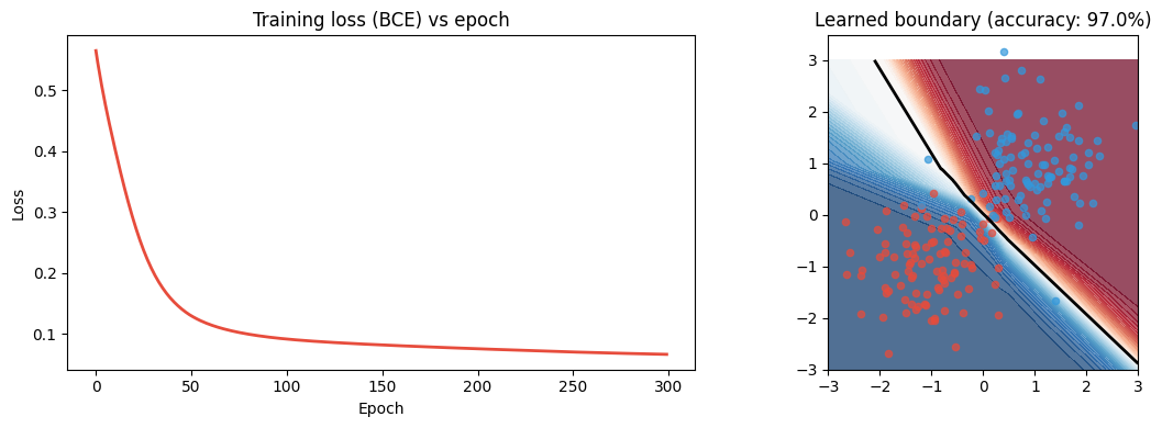

Final loss: 0.0667 | Accuracy: 97.0%

3. The computation graph view¶

Every operation in the forward pass is a node. Every edge carries a value forward and a gradient backward. Backprop is just topological sort + chain rule.

This is exactly what automatic differentiation (autograd) frameworks implement — PyTorch’s .backward(), JAX’s jax.grad(). The framework records the computation graph during the forward pass and traverses it in reverse on the backward pass.

(Automatic differentiation introduced conceptually in ch208.)

4. Vanishing and exploding gradients¶

At each layer: $dA^{[l-1]} = W^{[l]\top} \cdot dZ^{[l]}$ .

If $\|W^{[l]}\| < 1$ consistently, gradients shrink exponentially with depth → vanishing gradients. If $\|W^{[l]}\| > 1$ consistently → exploding gradients.

Mitigations:

Careful initialisation (ch308): set initial $\|W^{[l]}\|$ to avoid amplification or decay.
Batch normalisation (ch310): re-normalises activations mid-network.
Residual connections (ch316): bypass layers so gradients flow directly.
Gradient clipping (ch307): cap gradient norms before the update.

5. Summary¶

Backprop = chain rule applied in reverse topological order through the computation graph.
Three equations per layer: activation backward, weight gradient, bias gradient, upstream gradient.
The cache from the forward pass stores exactly what the backward pass needs.
Gradient checks (numerical vs analytical) verify the implementation is correct.
Vanishing/exploding gradients are structural risks addressed by init, normalisation, and architecture.

6. Forward and backward references¶

Used here: chain rule (ch215), partial derivatives (ch210), matrix transpose (ch154), forward pass and cache (ch304), loss gradients (ch305), activation derivatives (ch309).

This will reappear in ch316 — CNN Architectures, where backprop flows through convolutional layers (gradients are cross-correlations), and in ch337 — Transformer Block from Scratch, where attention gradients require careful handling of softmax Jacobians.