ch307 — Stochastic Gradient Descent - Mathematics for Programmers

1. Why stochastic?¶

Full-batch gradient descent computes the exact gradient over all $N$ training samples:

\nabla_\theta \mathcal{L} = \frac{1}{N}\sum_{i=1}^N \nabla_\theta \ell_i

(1)

This is expensive ( $O(N)$ per step) and offers no benefit once the gradient direction is well-estimated. Stochastic Gradient Descent (SGD) estimates the gradient from a mini-batch of $B \ll N$ samples:

\theta \leftarrow \theta - \eta \cdot \hat{g}_B, \quad \hat{g}_B = \frac{1}{B}\sum_{i \in \text{batch}} \nabla_\theta \ell_i

(2)

The estimate is noisy but unbiased: $\mathbb{E}[\hat{g}_B] = \nabla_\theta \mathcal{L}$ .

(Gradient descent: ch212. Expectation: ch249.)

2. Why noise helps¶

Counter-intuitively, gradient noise has benefits:

It escapes sharp minima (which tend to generalise poorly) and settles in flat minima (which tend to generalise well).
It prevents the optimiser from overfitting to noise in early training.
Theoretical analysis (Mandt et al., 2017) shows SGD noise acts as implicit regularisation.

3. SGD variants¶

Variant	Update rule	Key property
Vanilla SGD	$\theta \leftarrow \theta - \eta g$	Simple, no memory
SGD + Momentum	$v \leftarrow \mu v - \eta g$ ; $\theta \leftarrow \theta + v$	Dampens oscillation, accelerates
Nesterov	Lookahead gradient	Better convergence guarantees

Momentum accumulates a velocity vector $v$ , allowing the optimiser to accelerate in consistent gradient directions and slow down when direction oscillates.

(Adam and adaptive methods: ch312.)

import numpy as np
import matplotlib.pyplot as plt


def rosenbrock(params):
    """Classic test function: minimum at (1,1), banana-shaped valley."""
    x, y = params
    return (1 - x)**2 + 100 * (y - x**2)**2

def rosenbrock_grad(params):
    x, y = params
    dfdx = -2*(1 - x) - 400*x*(y - x**2)
    dfdy = 200*(y - x**2)
    return np.array([dfdx, dfdy])


def run_sgd(start, lr, momentum=0.0, n_steps=2000, noise=0.01, seed=0):
    rng = np.random.default_rng(seed)
    params = np.array(start, dtype=float)
    v = np.zeros_like(params)
    history = [params.copy()]
    for _ in range(n_steps):
        g = rosenbrock_grad(params) + rng.normal(0, noise, 2)  # simulate mini-batch noise
        v = momentum * v - lr * g
        params = params + v
        history.append(params.copy())
    return np.array(history)


configs = [
    ('SGD (no momentum)', 0.001, 0.0, '#e74c3c'),
    ('SGD + momentum 0.9', 0.001, 0.9, '#3498db'),
    ('SGD + momentum 0.99', 0.0005, 0.99, '#2ecc71'),
]

# Rosenbrock landscape
xs = np.linspace(-1.5, 1.5, 400)
ys = np.linspace(-0.5, 1.5, 400)
X, Y = np.meshgrid(xs, ys)
Z = (1 - X)**2 + 100*(Y - X**2)**2
Z_log = np.log1p(Z)

fig, axes = plt.subplots(1, 3, figsize=(15, 5))
start = [-1.0, 0.5]

for ax, (name, lr, mu, color) in zip(axes, configs):
    hist = run_sgd(start, lr, mu, n_steps=3000, noise=0.05)
    ax.contourf(X, Y, Z_log, levels=40, cmap='gray_r', alpha=0.8)
    ax.plot(hist[:, 0], hist[:, 1], color=color, lw=1.2, alpha=0.8)
    ax.scatter(*start, color='black', s=80, zorder=5, label='Start')
    ax.scatter(1, 1, color='gold', s=120, marker='*', zorder=5, label='Min (1,1)')
    ax.set_title(f'{name}\nfinal loss={rosenbrock(hist[-1]):.3f}')
    ax.set_xlim(-1.5, 1.5)
    ax.set_ylim(-0.5, 1.5)
    ax.legend(fontsize=8)

plt.suptitle('SGD variants on Rosenbrock function', fontsize=12)
plt.tight_layout()
plt.savefig('ch307_sgd.png', dpi=120)
plt.show()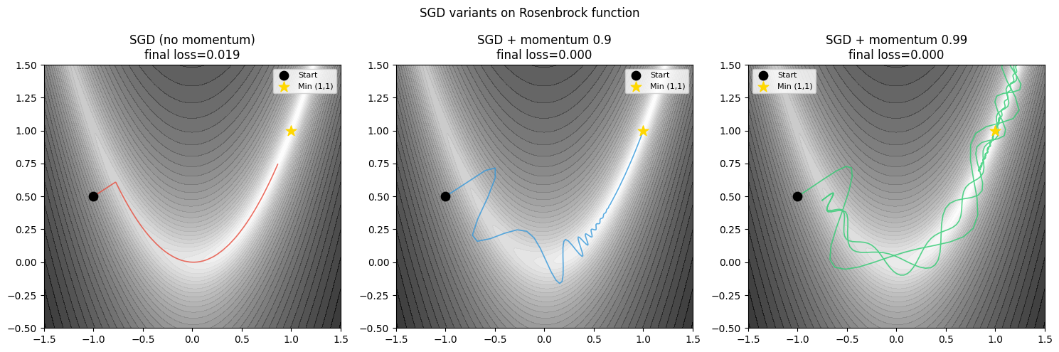

4. Practical SGD settings¶

Hyperparameter	Typical range	Effect
Learning rate $\eta$	0.001 – 0.1	Step size; most critical hyperparameter
Momentum $\mu$	0.9 – 0.99	Higher = more history, faster in smooth valleys
Batch size $B$	32 – 512	Larger = less noise, more parallelism, needs higher LR

Batch size scaling rule: When multiplying $B$ by $k$ , multiply $\eta$ by $\sqrt{k}$ (or linearly for short training runs). This keeps gradient noise variance constant.

5. Gradient clipping¶

For RNNs and deep networks, gradients can explode (ch306). Clipping caps gradient norm:

g \leftarrow g \cdot \min\left(1, \frac{\text{clip\_norm}}{\|g\|}\right)

(3)

This preserves direction while bounding magnitude. Common values: clip_norm = 1.0.

6. Summary¶

SGD uses mini-batch gradient estimates: unbiased, noisy, and computationally cheap.
Momentum accumulates gradient history to accelerate in consistent directions.
Batch size and learning rate are coupled: scaling one requires scaling the other.
Gradient clipping prevents explosions in deep/recurrent networks.

7. Forward and backward references¶

Used here: gradient descent (ch212), optimisation landscapes (ch213), backpropagation gradients (ch306), expectation (ch249).

This will reappear in ch312 — Optimisers: Adam, RMSProp, Momentum, where adaptive learning rates eliminate the need to hand-tune $\eta$ per parameter, and in ch334 — Project: Neural Net from Scratch, where SGD with momentum is implemented end-to-end.