ch308 — Initialisation Strategies - Mathematics for Programmers

1. Why initialisation matters¶

Backpropagation propagates gradients multiplicatively through $L$ layers. If weights are too large, activations and gradients explode. Too small, they vanish. Both pathologies kill learning (ch306, vanishing/exploding gradients).

The goal of initialisation is to set initial weights such that the variance of activations and gradients is approximately preserved across layers at the start of training.

2. The variance propagation analysis¶

For a linear layer $z = Wx$ with $n_{in}$ inputs, $n_{out}$ outputs, and $x \sim \mathcal{N}(0, 1)$ :

\text{Var}(z_i) = n_{in} \cdot \text{Var}(W_{ij}) \cdot \text{Var}(x_j)

(1)

To keep $\text{Var}(z) = \text{Var}(x)$ , we need $\text{Var}(W) = 1/n_{in}$ .

During backprop, the same analysis applies to gradients flowing backward, requiring $\text{Var}(W) = 1/n_{out}$ .

Xavier (Glorot) initialisation compromises between forward and backward:

W \sim \mathcal{U}\left(-\sqrt{\frac{6}{n_{in}+n_{out}}}, \sqrt{\frac{6}{n_{in}+n_{out}}}\right)

(2)

(Variance and distributions: ch250, ch253.)

import numpy as np
import matplotlib.pyplot as plt


def xavier_init(fan_in, fan_out, rng):
    limit = np.sqrt(6.0 / (fan_in + fan_out))
    return rng.uniform(-limit, limit, (fan_out, fan_in))

def he_init(fan_in, fan_out, rng):
    """He (Kaiming) initialisation for ReLU networks."""
    std = np.sqrt(2.0 / fan_in)
    return rng.normal(0, std, (fan_out, fan_in))

def naive_init(fan_in, fan_out, rng):
    return rng.normal(0, 0.01, (fan_out, fan_in))


def simulate_forward_variance(init_fn, layer_sizes, n_samples=1000, seed=0):
    """Track activation std across layers."""
    rng = np.random.default_rng(seed)
    x = rng.normal(0, 1, (layer_sizes[0], n_samples))
    stds = [x.std()]
    for i in range(len(layer_sizes) - 1):
        W = init_fn(layer_sizes[i], layer_sizes[i+1], rng)
        x = np.maximum(0, W @ x)  # ReLU
        stds.append(x.std())
    return stds


layer_sizes = [512] * 11  # 10 hidden layers

fig, axes = plt.subplots(1, 2, figsize=(12, 5))

for init_fn, name, color in [
    (naive_init, 'Naive (std=0.01)', '#e74c3c'),
    (xavier_init, 'Xavier', '#f39c12'),
    (he_init, 'He (for ReLU)', '#2ecc71'),
]:
    stds = simulate_forward_variance(init_fn, layer_sizes)
    axes[0].plot(stds, marker='o', color=color, label=name)

axes[0].set_title('Activation std across 10 layers\n(ReLU activations)')
axes[0].set_xlabel('Layer')
axes[0].set_ylabel('Std of activations')
axes[0].set_yscale('log')
axes[0].legend()
axes[0].axhline(1.0, color='black', linestyle='--', alpha=0.4, label='Target std=1')

# Distribution of activations at layer 5
for init_fn, name, color in [
    (naive_init, 'Naive', '#e74c3c'),
    (xavier_init, 'Xavier', '#f39c12'),
    (he_init, 'He', '#2ecc71'),
]:
    rng = np.random.default_rng(0)
    x = rng.normal(0, 1, (512, 500))
    for i in range(5):
        W = init_fn(512, 512, rng)
        x = np.maximum(0, W @ x)
    axes[1].hist(x.ravel()[:3000], bins=60, alpha=0.5, color=color, label=name, density=True)

axes[1].set_title('Activation distribution at layer 5')
axes[1].set_xlabel('Activation value')
axes[1].set_ylabel('Density')
axes[1].legend()

plt.suptitle('Initialisation strategy determines whether activations survive depth', fontsize=11)
plt.tight_layout()
plt.savefig('ch308_init.png', dpi=120)
plt.show()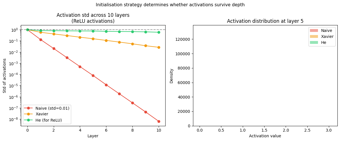

3. He initialisation for ReLU¶

Xavier assumes symmetric activations. ReLU kills half the variance (negative half → 0). He (Kaiming) initialisation corrects for this:

W \sim \mathcal{N}\left(0, \sqrt{\frac{2}{n_{in}}}\right)

(3)

The factor of 2 compensates for the expected 50% dead neurons at each layer.

Use Xavier for Tanh/Sigmoid activations. Use He for ReLU and its variants.

4. Orthogonal initialisation¶

For very deep networks, random initialisation can still cause issues. Orthogonal initialisation sets $W$ to a random orthogonal matrix (via QR decomposition of a random Gaussian matrix). Orthogonal matrices preserve vector norms exactly: $\|Wx\| = \|x\|$ .

This guarantees neither explosion nor vanishing at initialisation, but requires the matrix to be square — impractical for arbitrary layer sizes. Used in RNNs (ch317).

5. Bias initialisation¶

Biases are almost always initialised to zero. The exception: output layer biases can be set to $\log(p/(1-p))$ where $p$ is the base rate of the positive class — this speeds up early convergence for imbalanced datasets.

6. Summary¶

Variance must be preserved across layers: too large = explosion, too small = vanishing.
Xavier: correct for tanh/sigmoid. He: correct for ReLU (factor of 2 for killed half).
Bias initialisation: zero, unless you have domain knowledge about base rates.
Orthogonal init: useful for RNNs and very deep networks.

7. Forward and backward references¶

Used here: variance (ch250), normal distribution (ch253), chain rule through layers (ch306).

This will reappear in ch310 — Batch Normalisation, which eliminates much of the sensitivity to initialisation by normalising activations during training.