Chapter 45 — Computational Logarithms

# --- Visualization: Taylor series approximation of ln(1+u) ---
import numpy as np
import matplotlib.pyplot as plt

plt.style.use('seaborn-v0_8-whitegrid')

u = np.linspace(-0.99, 1.5, 400)
exact = np.log1p(u)  # exact ln(1+u)

# Partial sums of Taylor series: sum_{k=1}^{N} (-1)^(k+1) u^k / k
def taylor_ln1p(u, N):
    """Compute ln(1+u) via Taylor series with N terms."""
    result = np.zeros_like(u, dtype=float)
    for k in range(1, N + 1):
        result += ((-1)**(k+1)) * u**k / k
    return result

fig, axes = plt.subplots(1, 2, figsize=(13, 5))

ax = axes[0]
ax.plot(u, exact, 'k-', linewidth=2.5, label='Exact: ln(1+u)', zorder=10)
for N, color in [(1, 'red'), (2, 'orange'), (4, 'blue'), (10, 'green')]:
    approx = taylor_ln1p(u, N)
    ax.plot(u, approx, linestyle='--', color=color, label=f'{N} terms', alpha=0.8)
ax.set_ylim(-3, 3)
ax.axvline(0, color='gray', linewidth=0.5)
ax.axhline(0, color='gray', linewidth=0.5)
ax.set_title('Taylor Series Approximation of ln(1+u)')
ax.set_xlabel('u')
ax.set_ylabel('ln(1+u)')
ax.legend(fontsize=9)

# Error plot — only for u in (-1, 1)
u_safe = np.linspace(-0.99, 0.99, 400)
exact_safe = np.log1p(u_safe)
ax = axes[1]
for N, color in [(1, 'red'), (2, 'orange'), (4, 'blue'), (8, 'green'), (16, 'purple')]:
    err = np.abs(taylor_ln1p(u_safe, N) - exact_safe)
    ax.semilogy(u_safe, err + 1e-17, color=color, label=f'{N} terms')
ax.set_title('Approximation Error vs Number of Terms')
ax.set_xlabel('u')
ax.set_ylabel('|Error| (log scale)')
ax.legend(fontsize=9)

plt.tight_layout()
plt.show()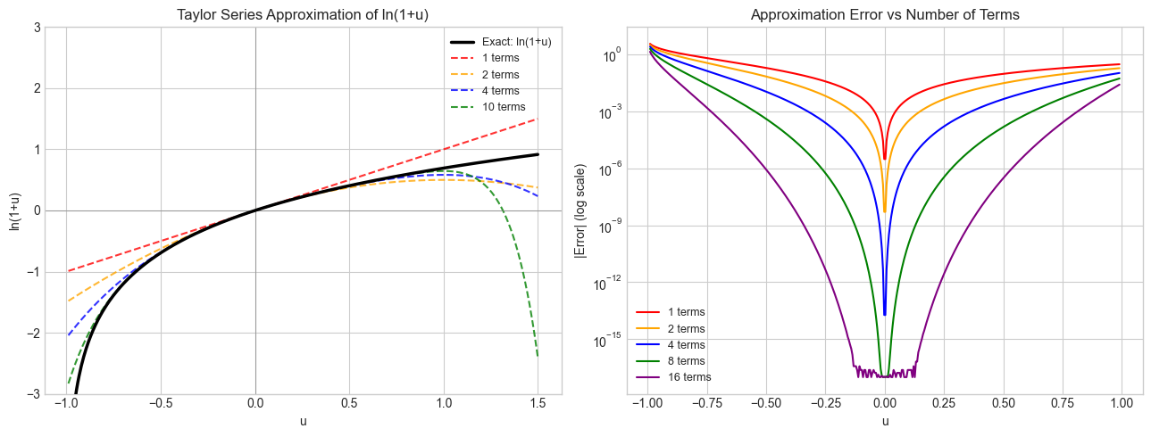

# --- Visualization: Range reduction — decomposing any x into mantissa and exponent ---
import numpy as np
import matplotlib.pyplot as plt

plt.style.use('seaborn-v0_8-whitegrid')

# Show how range reduction maps various x values to their (n, m) components
test_values = [0.125, 0.5, 1.0, 1.5, 2.0, 4.7, 8.0, 100.0, 0.001]

print("Range Reduction: x = 2^n × m, where 1 ≤ m < 2")
print(f"{'x':>10} {'n':>5} {'m':>10} {'n×ln2':>12} {'ln(m)':>12} {'sum=ln(x)':>14} {'np.log(x)':>14}")
print("-" * 80)

LN2 = np.log(2)
for x in test_values:
    # Extract n and m using Python's frexp: returns (m, n) with x = m * 2^n, 0.5 ≤ m < 1
    import math
    m_frac, n = math.frexp(x)  # note: frexp gives 0.5 <= m < 1, not 1 <= m < 2
    # Adjust to get 1 ≤ m < 2
    m = m_frac * 2
    n = n - 1
    ln_x_via_reduction = n * LN2 + np.log(m)
    ln_x_exact = np.log(x)
    print(f"{x:>10.4f} {n:>5} {m:>10.6f} {n*LN2:>12.6f} {np.log(m):>12.6f} {ln_x_via_reduction:>14.8f} {ln_x_exact:>14.8f}")

print("\nAll m values are in [1, 2) — well within the Taylor series radius of convergence.")

# --- Implementation: ln(x) via Taylor series + range reduction ---
import numpy as np
import math

LN2 = 0.6931471805599453  # ln(2), known constant

def ln_taylor(u, n_terms=50):
    """
    Compute ln(1 + u) via Taylor series.
    ln(1+u) = u - u^2/2 + u^3/3 - u^4/4 + ...

    Converges for |u| < 1.

    Args:
        u:       value with |u| < 1
        n_terms: number of Taylor series terms

    Returns:
        Approximate ln(1+u)
    """
    if abs(u) >= 1:
        raise ValueError("|u| must be < 1 for convergence")
    result = 0.0
    u_power = u  # u^k, starting at k=1
    for k in range(1, n_terms + 1):
        result += ((-1)**(k+1)) * u_power / k
        u_power *= u
    return result


def ln_from_scratch(x, n_terms=60):
    """
    Compute ln(x) for x > 0 using range reduction + Taylor series.

    Steps:
      1. Extract mantissa m and exponent n from x = m × 2^n  (1 ≤ m < 2)
      2. ln(x) = n × ln(2) + ln(m) = n × ln(2) + ln(1 + (m-1))
      3. Apply Taylor series with u = m - 1

    Args:
        x:       positive real number
        n_terms: Taylor series terms for ln(m)

    Returns:
        Approximate ln(x)
    """
    if x <= 0:
        raise ValueError("ln undefined for x <= 0")

    # Range reduction via frexp
    m_frac, exp_n = math.frexp(x)  # x = m_frac × 2^exp_n, 0.5 ≤ m_frac < 1
    m = m_frac * 2                  # shift to [1, 2)
    n = exp_n - 1                   # adjust exponent

    # u = m - 1 is in [0, 1)
    u = m - 1
    ln_m = ln_taylor(u, n_terms)

    return n * LN2 + ln_m


# Validate
test_vals = [0.001, 0.1, 0.5, 1.0, 2.0, np.e, 10.0, 100.0, 1e6]
print(f"{'x':>12} {'ln_from_scratch':>18} {'np.log(x)':>18} {'abs_error':>16}")
print("-" * 68)
for x in test_vals:
    ours = ln_from_scratch(x)
    ref  = math.log(x)
    err  = abs(ours - ref)
    print(f"{x:>12.4f} {ours:>18.10f} {ref:>18.10f} {err:>16.2e}")

# --- Implementation: Newton's method for ln(x) ---
import numpy as np
import math

def ln_newton(x, n_iter=10):
    """
    Compute ln(x) via Newton's method applied to f(y) = e^y - x = 0.

    Update: y_{k+1} = y_k - 1 + x / e^{y_k}

    Initial guess: use range reduction to get a ballpark value.

    Args:
        x:      positive real number
        n_iter: number of Newton iterations

    Returns:
        Approximate ln(x)
    """
    if x <= 0:
        raise ValueError("ln undefined for x <= 0")

    # Initial guess: use bit_length approximation
    # If x ≈ 2^n, then ln(x) ≈ n × ln(2)
    y = math.floor(math.log2(x)) * 0.693  # rough estimate

    for _ in range(n_iter):
        ey = math.exp(y)
        y = y - 1 + x / ey  # Newton update

    return y


print("Newton's method convergence for ln(7.389):")
target = np.e**2  # ≈ 7.389, so ln = 2
print(f"True value: {math.log(target):.12f}")
print()

y = math.floor(math.log2(target)) * 0.693
for i in range(8):
    ey = math.exp(y)
    y  = y - 1 + target / ey
    err = abs(y - math.log(target))
    print(f"  Iter {i+1}: y={y:.12f}  error={err:.2e}")

# --- Experiment 1: The log1p problem — cancellation in naive computation ---
# Hypothesis: For small x, log(1+x) via naive computation loses all precision.
# log1p(x) avoids this. The crossover is around x = 1e-8.
# Try changing: X_MIN_EXP to see the boundary

import numpy as np

X_MIN_EXP = -18  # <-- modify this (try -14, -20)

print(f"{'x':>12} {'log(1+x) naive':>18} {'log1p(x)':>18} {'diff':>14}")
print("-" * 65)
for exp in range(0, X_MIN_EXP - 1, -2):
    x = 10**exp
    naive = np.log(1 + x)
    safe  = np.log1p(x)
    diff  = abs(naive - safe)
    print(f"{x:>12.0e} {naive:>18.10e} {safe:>18.10e} {diff:>14.2e}")

print("\nFor x < ~1e-8, naive computation returns 0.0 — total loss of precision.")
print("np.log1p(x) uses the Taylor expansion directly: ~x for tiny x.")

# --- Experiment 2: How many Taylor terms are needed for float64 precision? ---
# Hypothesis: Near u = 0.99 (boundary of convergence), many more terms
# are needed than near u = 0.1.
# Try changing: U_TEST

import numpy as np

U_TEST = 0.9   # <-- modify this (try 0.1, 0.5, 0.99, -0.9)
FLOAT64_EPS = 2.2e-16

print(f"Taylor series accuracy for u = {U_TEST}")
print(f"Target: ln(1 + {U_TEST}) = {np.log1p(U_TEST):.15f}")
print()
print(f"{'N terms':>10} {'approximation':>20} {'error':>15} {'digits correct':>15}")
print("-" * 65)

exact = np.log1p(U_TEST)
for N in [1, 2, 5, 10, 20, 50, 100, 200]:
    approx = sum(((-1)**(k+1)) * U_TEST**k / k for k in range(1, N+1))
    err = abs(approx - exact)
    digits = int(-np.log10(err + 1e-320))
    converged = '✓' if err < FLOAT64_EPS else ''
    print(f"{N:>10} {approx:>20.12f} {err:>15.2e} {digits:>15}  {converged}")

# --- Experiment 3: Speed comparison — Taylor series vs Newton's method ---
# Hypothesis: Newton's method converges in far fewer iterations than Taylor series
# for inputs far from u=0, because it converges quadratically.

import numpy as np
import math

TARGET = 1000.0  # <-- modify this (try 0.001, 1e10)
TRUE   = math.log(TARGET)
EPS    = 1e-14

print(f"Computing ln({TARGET}) = {TRUE:.10f}")
print(f"Target precision: {EPS:.1e}")
print()

# Taylor series: must use range reduction first, then count terms for ln(m)
m_frac, exp_n = math.frexp(TARGET)
m = m_frac * 2; n = exp_n - 1
u = m - 1
LN2 = 0.6931471805599453
result = 0.0
u_power = u
for k in range(1, 201):
    term = ((-1)**(k+1)) * u_power / k
    result += term
    u_power *= u
    approx_ln = n * LN2 + result
    if abs(approx_ln - TRUE) < EPS:
        print(f"Taylor (with range reduction): converged in {k} terms for ln(m)")
        print(f"  m = {m:.6f}, u = {u:.6f}, n = {n}")
        break

# Newton's method
y = math.floor(math.log2(TARGET)) * 0.693
for i in range(30):
    ey = math.exp(y)
    y  = y - 1 + TARGET / ey
    if abs(y - TRUE) < EPS:
        print(f"Newton's method: converged in {i+1} iterations")
        break

# --- Mini Project: A self-contained log/exp module ---
#
# Problem:
#   Build a minimal `mymath` module that can compute log, exp, and pow
#   for positive real numbers without using math or numpy's log/exp functions.
#   Use only: +, -, *, /, Python integers, and math.frexp/math.ldexp.
#
# This is the kind of problem that library developers actually solve.

import math

# --- Constants (computed to full precision using the known series) ---
# We allow ourselves to use these pre-computed values.
LN2 = 0.6931471805599453
LN10 = 2.302585092994046
E    = 2.718281828459045


def myexp(x, n_terms=60):
    """
    Compute e^x via Taylor series: e^x = sum_{k=0}^{inf} x^k / k!

    Range reduction: write x = n + f where n = floor(x), f = x - n ∈ [0,1)
    Then e^x = e^n × e^f ≈ E^n × taylor(f)
    """
    # Handle sign: e^x = 1 / e^(-x)
    if x < 0:
        return 1.0 / myexp(-x, n_terms)

    # Range reduction: separate integer and fractional parts
    n = int(x)
    f = x - n

    # Taylor series for e^f (f ∈ [0, 1))
    result = 1.0      # k=0 term
    term   = 1.0      # running term: f^k / k!
    for k in range(1, n_terms + 1):
        term *= f / k
        result += term
        if abs(term) < 1e-17:
            break

    # Multiply by e^n = E^n
    e_to_n = 1.0
    for _ in range(n):
        e_to_n *= E

    return e_to_n * result


def mylog(x):
    """Compute ln(x) via range reduction + arctanh series (fast)."""
    if x <= 0:
        raise ValueError("ln undefined for x <= 0")

    # Range reduction via frexp
    m_frac, exp_n = math.frexp(x)
    m = m_frac * 2
    n = exp_n - 1

    # ln(m) via arctanh identity: ln(m) = 2 * arctanh((m-1)/(m+1))
    t = (m - 1) / (m + 1)  # t ∈ [0, 1/3) for m ∈ [1, 2)
    t2 = t * t
    atanh = t
    term  = t
    for k in range(1, 60):
        term  *= t2
        contrib = term / (2 * k + 1)
        atanh += contrib
        if abs(contrib) < 1e-17:
            break
    ln_m = 2 * atanh

    return n * LN2 + ln_m


def mypow(base, exp):
    """
    Compute base^exp for base > 0, real exp.
    Uses: base^exp = e^(exp × ln(base))
    """
    if base <= 0:
        raise ValueError("base must be positive for real exponents")
    return myexp(exp * mylog(base))


# --- Validation ---
import numpy as np

test_x = [0.001, 0.1, 0.5, 1.0, 2.0, 7.389, 100.0, 1e6]
print("=== mylog vs math.log ===")
print(f"{'x':>10} {'mylog':>16} {'math.log':>16} {'error':>12}")
for x in test_x:
    v = mylog(x); ref = math.log(x)
    print(f"{x:>10.4f} {v:>16.10f} {ref:>16.10f} {abs(v-ref):>12.2e}")

print("\n=== myexp vs math.exp ===")
print(f"{'x':>10} {'myexp':>16} {'math.exp':>16} {'error':>12}")
for x in [-3, -1, 0, 0.5, 1, 2, 5, 10]:
    v = myexp(x); ref = math.exp(x)
    print(f"{x:>10.2f} {v:>16.8f} {ref:>16.8f} {abs(v-ref):>12.2e}")

print("\n=== mypow vs ** ===")
print(f"{'b^e':>14} {'mypow':>16} {'b**e':>16} {'error':>12}")
for b, e in [(2, 10), (3, 0.5), (10, 3.14), (np.e, 2.5)]:
    v = mypow(b, e); ref = b**e
    print(f"{b}^{e:>6} = {v:>16.8f} {ref:>16.8f} {abs(v-ref):>12.2e}")