Prerequisites: ch041 (Exponents and Powers), ch042 (Exponential Growth), ch043 (Logarithms Intuition), ch044 (Logarithmic Scales)
You will learn:
The hierarchy of growth rates: constant < log < polynomial < exponential < factorial
Formal asymptotic notation: O, Ω, Θ, and how to use it correctly
Why the growth hierarchy matters far more than constant factors for large inputs
How to compare two growth rates rigorously using limits
Stirling’s approximation for factorial growth
Environment: Python 3.x, numpy, matplotlib
1. Concept
When an algorithm runs in O(n²) time, and a competitor’s runs in O(n log n), which is faster? “It depends on the constant factor” — but only for small n. For large n, the growth rate dominates everything else.
The fundamental growth hierarchy (slowest to fastest):
O(1) < O(log n) < O(√n) < O(n) < O(n log n) < O(n²) < O(n³) < O(2ⁿ) < O(n!)Every function in this list eventually dominates all functions to its left — no matter how large the constant factors.
What this means in practice:
A
O(2^n)algorithm with constant factor 0.0001 is eventually slower than aO(n^1000)algorithm with constant factor 10^100.Eventually. The crossover point might be at
n = 10^50, but the hierarchy is strict.
Why it matters: Algorithm selection, data structure choice, feasibility analysis, and understanding which mathematical operations are “cheap” vs “expensive” all depend on understanding where operations fall in this hierarchy.
Common misconception: O-notation describes worst-case behavior in many (but not all) contexts. It also describes average case, best case, or expected case — the notation itself says nothing about which. Always state what case you’re analyzing.
2. Intuition & Mental Models
Physical analogy: Think of different growth rates as different transportation modes. Constant time is teleportation — you’re already there. Log time is a subway (each station covers 2× the distance). Linear is walking. Polynomial is crawling. Exponential is running backwards.
Computational analogy: Think of growth rate as “how does problem difficulty change when you double the input?”:
O(1): no change — sorting a million items takes the same time as sorting 1 if you have a hash table lookup.O(log n): adds one step — binary search on 2n items takes 1 step more.O(n): doubles — processing 2n items takes 2× as long.O(n²): quadruples — 2n items → 4× as long.O(2^n): squares — 2(n+1) = 2×2^n, so adding one input doubles the work.
The limit tool: To compare f(n) vs g(n), compute lim_{n→∞} f(n)/g(n):
Result = 0:
fgrows slower thang(f = o(g))Result = c > 0 (finite): same growth rate (
f = Θ(g))Result = ∞:
fgrows faster thang
Recall from ch042: Exponential growth overtakes any polynomial (from ch042 — Exponential Growth). The ratio 2^n / n^k → ∞ for any fixed k.
3. Visualization
# --- Visualization: The growth hierarchy ---
import numpy as np
import matplotlib.pyplot as plt

plt.style.use('seaborn-v0_8-whitegrid')

n = np.linspace(1, 30, 500)

growth_functions = [
    ('O(1)',      np.ones_like(n),               'black'),
    ('O(log n)',  np.log2(n),                     'green'),
    ('O(√n)',     np.sqrt(n),                     'lime'),
    ('O(n)',      n,                              'blue'),
    ('O(n log n)', n * np.log2(n),               'purple'),
    ('O(n²)',     n**2,                           'orange'),
    ('O(2ⁿ)',     2**n,                           'red'),
]

fig, axes = plt.subplots(1, 2, figsize=(14, 6))

for label, f, color in growth_functions:
    axes[0].plot(n, f, label=label, color=color, linewidth=1.8)
    safe = f[f > 0]
    n_safe = n[f > 0]
    axes[1].semilogy(n_safe, safe, label=label, color=color, linewidth=1.8)

axes[0].set_ylim(0, 200)
axes[0].set_title('Growth Functions (Linear Scale, capped at 200)')
axes[0].set_xlabel('n')
axes[0].set_ylabel('f(n)')
axes[0].legend(fontsize=9)

axes[1].set_title('Growth Functions (Semilog Scale)')
axes[1].set_xlabel('n')
axes[1].set_ylabel('f(n) [log scale]')
axes[1].legend(fontsize=9)

plt.suptitle('The Growth Rate Hierarchy', fontsize=14)
plt.tight_layout()
plt.show()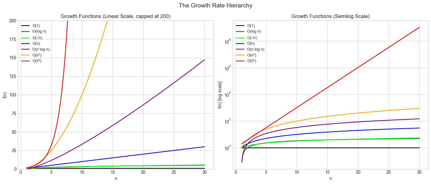
# --- Visualization: Crossover points — when does faster eventually win? ---
import numpy as np
import matplotlib.pyplot as plt

plt.style.use('seaborn-v0_8-whitegrid')

# Case: Algorithm A (fast constant, worse complexity) vs Algorithm B (slow constant, better complexity)
n = np.linspace(1, 100, 500)

A_const, A_growth = 1.0, lambda n: n**2      # O(n²)
B_const, B_growth = 100.0, lambda n: n       # O(n), but 100× slower constant

f_A = A_const * A_growth(n)
f_B = B_const * B_growth(n)

fig, ax = plt.subplots(figsize=(10, 5))
ax.plot(n, f_A, label='A: 1.0 × n²  [O(n²)]',  color='red',  linewidth=2)
ax.plot(n, f_B, label='B: 100 × n   [O(n)]',    color='blue', linewidth=2)

# Find crossover: f_A = f_B → n² = 100n → n = 100
crossover = 100
ax.axvline(crossover, color='gray', linestyle='--', linewidth=1)
ax.annotate(f'Crossover at n={crossover}', (crossover, f_A[np.argmin(np.abs(n-crossover))]),
            xytext=(60, 5000), fontsize=10, arrowprops=dict(arrowstyle='->'))

ax.fill_between(n, f_A, f_B, where=f_A < f_B, alpha=0.1, color='red',  label='A faster')
ax.fill_between(n, f_A, f_B, where=f_A >= f_B, alpha=0.1, color='blue', label='B faster')

ax.set_title('Crossover: Better Growth Rate Eventually Wins\n(even with 100× worse constant factor)')
ax.set_xlabel('Input size n')
ax.set_ylabel('Operations')
ax.legend()
ax.set_ylim(0, 10000)
plt.tight_layout()
plt.show()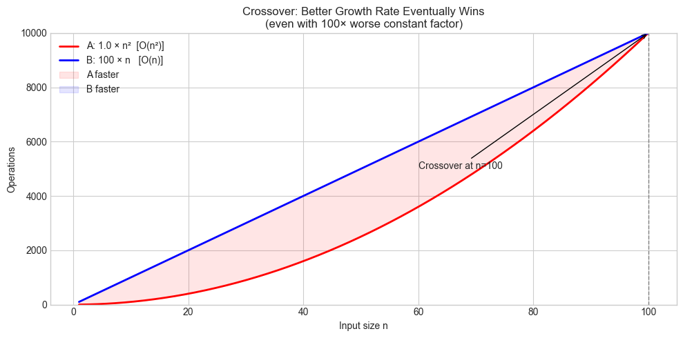
4. Mathematical Formulation
Asymptotic notation
f(n) = O(g(n)):  there exist C > 0, n₀ > 0 such that f(n) ≤ C·g(n) for all n > n₀
                 "f is eventually bounded above by a constant multiple of g"

f(n) = Ω(g(n)):  there exist C > 0, n₀ > 0 such that f(n) ≥ C·g(n) for all n > n₀
                 "f grows at least as fast as g"

f(n) = Θ(g(n)):  f = O(g) AND f = Ω(g)
                 "f and g grow at the same rate (same order)"

f(n) = o(g(n)):  lim_{n→∞} f(n)/g(n) = 0
                 "f grows strictly slower than g"
The limit comparison
lim_{n→∞} f(n)/g(n) = 0   →  f = o(g)    (f grows slower)
lim_{n→∞} f(n)/g(n) = L>0 →  f = Θ(g)   (same rate)
lim_{n→∞} f(n)/g(n) = ∞   →  f = ω(g)   (f grows faster)
Stirling’s approximation
Factorial growth is faster than exponential:
n! ≈ √(2πn) × (n/e)^n

ln(n!) ≈ n·ln(n) - n + (1/2)·ln(2πn)
This shows n! grows faster than a^n for any base a — the exponent in (n/e)^n itself grows with n.
Key limit results to know
lim n^k / a^n = 0     for any k, a > 1     (exponential beats polynomial)
lim (log n)^k / n = 0 for any k > 0        (polynomial beats any power of log)
lim a^n / n! = 0      for any a             (factorial beats exponential)
# --- Verify limit claims numerically ---
import numpy as np
print("Limit verification: ratios as n → ∞")
print("\n1. n^k / 2^n → 0 (exponential beats polynomial)")
for k in [2, 5, 10]:
ratios = [(n, n**k / 2**n) for n in [10, 50, 100, 200]]
row = " " + " ".join(f"n={n}: {r:.2e}" for n, r in ratios)
print(f" k={k:2d}: {row}")
print("\n2. (log n)^k / n → 0 (n beats any power of log n)")
for k in [1, 2, 5]:
ratios = [(n, np.log(n)**k / n) for n in [100, 10_000, 1_000_000]]
row = " " + " ".join(f"n={n:.0e}: {r:.2e}" for n, r in ratios)
print(f" k={k}: {row}")
print("\n3. 2^n / n! → 0 (factorial beats exponential)")
import math
for n in [5, 10, 20, 30, 40]:
r = 2**n / math.factorial(n)
print(f" n={n:2d}: 2^n / n! = {r:.4e}")Limit verification: ratios as n → ∞
1. n^k / 2^n → 0 (exponential beats polynomial)
k= 2: n=10: 9.77e-02 n=50: 2.22e-12 n=100: 7.89e-27 n=200: 2.49e-56
k= 5: n=10: 9.77e+01 n=50: 2.78e-07 n=100: 7.89e-21 n=200: 1.99e-49
k=10: n=10: 9.77e+06 n=50: 8.67e+01 n=100: 7.89e-11 n=200: 6.37e-38
2. (log n)^k / n → 0 (n beats any power of log n)
k=1: n=1e+02: 4.61e-02 n=1e+04: 9.21e-04 n=1e+06: 1.38e-05
k=2: n=1e+02: 2.12e-01 n=1e+04: 8.48e-03 n=1e+06: 1.91e-04
k=5: n=1e+02: 2.07e+01 n=1e+04: 6.63e+00 n=1e+06: 5.03e-01
3. 2^n / n! → 0 (factorial beats exponential)
n= 5: 2^n / n! = 2.6667e-01
n=10: 2^n / n! = 2.8219e-04
n=20: 2^n / n! = 4.3100e-13
n=30: 2^n / n! = 4.0480e-24
n=40: 2^n / n! = 1.3476e-36
5. Python Implementation
# --- Implementation: Growth rate comparison tool ---
import numpy as np
import math
import matplotlib.pyplot as plt

plt.style.use('seaborn-v0_8-whitegrid')

def compare_growth_rates(f, g, f_label, g_label, n_values=None):
    """
    Compare two growth functions f(n) and g(n) by computing their ratio.

    If ratio → 0:   f is o(g) — f grows slower
    If ratio → L>0: f is Θ(g) — same order
    If ratio → ∞:   f is ω(g) — f grows faster

    Args:
        f, g:         callables taking a numpy array
        f_label, g_label: names for display
        n_values:     array of n values to evaluate

    Returns:
        Ratio array f(n)/g(n)
    """
    if n_values is None:
        n_values = np.logspace(0, 4, 400)

    f_vals = f(n_values)
    g_vals = g(n_values)

    # Avoid division by zero
    ratio = np.where(g_vals > 0, f_vals / g_vals, np.nan)

    fig, axes = plt.subplots(1, 2, figsize=(13, 5))

    ax = axes[0]
    ax.loglog(n_values, f_vals, label=f_label, color='blue')
    ax.loglog(n_values, g_vals, label=g_label, color='red')
    ax.set_title(f'{f_label} vs {g_label}')
    ax.set_xlabel('n (log scale)')
    ax.set_ylabel('f(n) (log scale)')
    ax.legend()

    ax = axes[1]
    finite = np.isfinite(ratio) & (ratio > 0)
    ax.semilogx(n_values[finite], ratio[finite], color='green', linewidth=2)
    ax.axhline(0, color='gray', linestyle='--', linewidth=0.8)
    ax.set_title(f'Ratio: f(n) / g(n)   [{f_label} / {g_label}]')
    ax.set_xlabel('n (log scale)')
    ax.set_ylabel('ratio')

    plt.tight_layout()
    plt.show()

    # Report the ratio at the largest n
    last_ratio = ratio[finite][-1] if finite.any() else float('nan')
    print(f"Ratio at n={n_values[finite][-1]:.0f}: {last_ratio:.6f}")
    if last_ratio < 0.01:
        print(f"  → {f_label} = o({g_label})  (f grows slower)")
    elif last_ratio > 100:
        print(f"  → {f_label} = ω({g_label})  (f grows faster)")
    else:
        print(f"  → {f_label} = Θ({g_label})  (same order)")

    return ratio


# Example: n log n vs n^1.1 — which grows faster?
n_vals = np.linspace(2, 10_000, 1000)
ratio = compare_growth_rates(
    f=lambda n: n * np.log2(n),
    g=lambda n: n**1.1,
    f_label='n log n',
    g_label='n^1.1',
    n_values=n_vals
)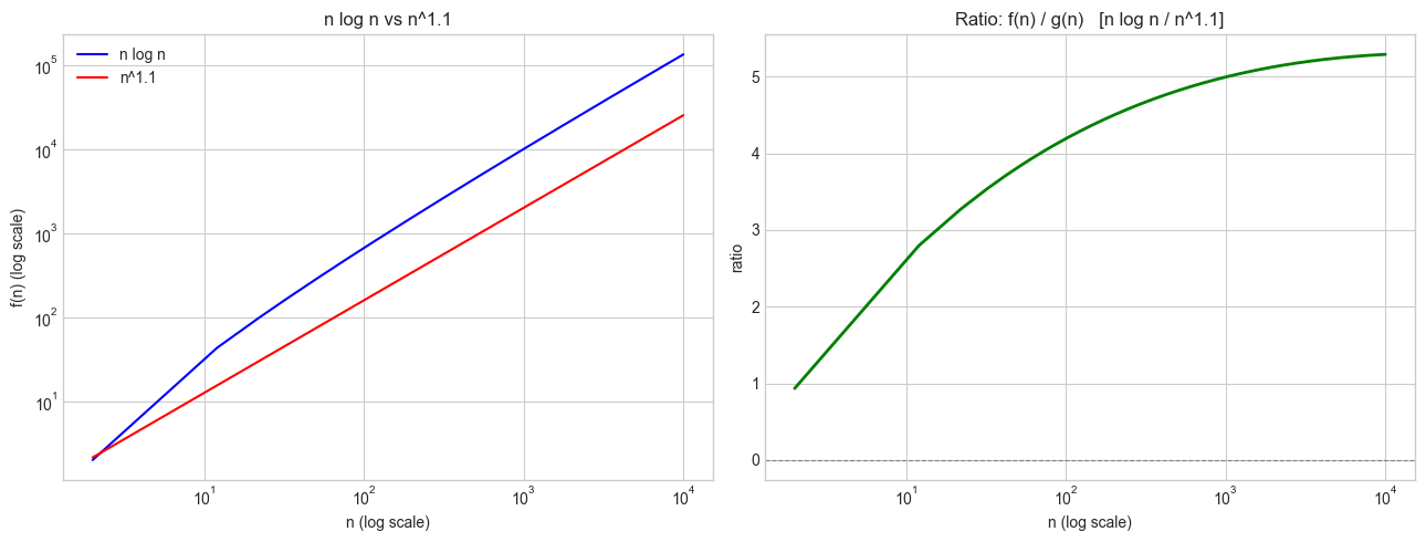
Ratio at n=10000: 5.289934
  → n log n = Θ(n^1.1)  (same order)
6. Experiments
# --- Experiment 1: Stirling's approximation accuracy ---
# Hypothesis: Stirling's approximation becomes extremely accurate as n grows.
# The relative error decreases as 1/(12n).
# Try changing: MAX_N

import numpy as np
import math

MAX_N = 30  # <-- modify this (try 50, 100)

print(f"Stirling's approximation: n! ≈ √(2πn) × (n/e)^n")
print(f"{'n':>5} {'n!':>20} {'Stirling':>20} {'rel error':>12}")
print("-" * 62)

for n in range(1, MAX_N + 1):
    exact    = float(math.factorial(n))
    stirling = math.sqrt(2 * math.pi * n) * (n / math.e) ** n
    rel_err  = abs(exact - stirling) / exact
    if n <= 10 or n % 5 == 0:
        print(f"{n:>5} {exact:>20.4e} {stirling:>20.4e} {rel_err:>12.4e}")
Stirling's approximation: n! ≈ √(2πn) × (n/e)^n
n n! Stirling rel error
--------------------------------------------------------------
1 1.0000e+00 9.2214e-01 7.7863e-02
2 2.0000e+00 1.9190e+00 4.0498e-02
3 6.0000e+00 5.8362e+00 2.7298e-02
4 2.4000e+01 2.3506e+01 2.0576e-02
5 1.2000e+02 1.1802e+02 1.6507e-02
6 7.2000e+02 7.1008e+02 1.3780e-02
7 5.0400e+03 4.9804e+03 1.1826e-02
8 4.0320e+04 3.9902e+04 1.0357e-02
9 3.6288e+05 3.5954e+05 9.2128e-03
10 3.6288e+06 3.5987e+06 8.2960e-03
15 1.3077e+12 1.3004e+12 5.5393e-03
20 2.4329e+18 2.4228e+18 4.1577e-03
25 1.5511e+25 1.5460e+25 3.3276e-03
30 2.6525e+32 2.6452e+32 2.7738e-03
# --- Experiment 2: n log n vs n^1.5 — a counterintuitive crossover ---
# Hypothesis: n^1.5 eventually dominates n log n because 1.5 > 1.
# But the crossover requires very large n.
# Try changing: EXPONENT to find when crossover happens

import numpy as np
import matplotlib.pyplot as plt

plt.style.use('seaborn-v0_8-whitegrid')

EXPONENT = 1.5   # <-- modify this (try 1.1, 1.2, 2.0)

n = np.logspace(0, 8, 500)  # 1 to 10^8

f = n * np.log2(np.maximum(n, 1))
g = n ** EXPONENT

ratio = f / g

# Find approximate crossover
crossover_idx = np.argwhere(ratio < 1)
crossover_n = n[crossover_idx[0][0]] if len(crossover_idx) > 0 else None

fig, ax = plt.subplots(figsize=(9, 5))
ax.semilogx(n, ratio, color='steelblue', linewidth=2)
ax.axhline(1, color='red', linestyle='--', label='ratio = 1 (equal)')
if crossover_n:
    ax.axvline(crossover_n, color='gray', linestyle='--', alpha=0.7,
               label=f'Crossover ≈ n={crossover_n:.1e}')
ax.set_title(f'Ratio: n·log₂n / n^{EXPONENT}  (→ 0 means n^{EXPONENT} dominates)')
ax.set_xlabel('n (log scale)')
ax.set_ylabel('Ratio')
ax.legend()
plt.tight_layout()
plt.show()

if crossover_n:
    print(f"n·log n is larger than n^{EXPONENT} until approximately n = {crossover_n:.2e}")
    print(f"For n > {crossover_n:.2e}: n^{EXPONENT} = ω(n log n)")
C:\Users\user\AppData\Local\Temp\ipykernel_13996\3775643615.py:34: UserWarning: Glyph 8322 (\N{SUBSCRIPT TWO}) missing from font(s) Arial.
plt.tight_layout()
c:\Users\user\OneDrive\Documents\book\.venv\Lib\site-packages\IPython\core\pylabtools.py:170: UserWarning: Glyph 8322 (\N{SUBSCRIPT TWO}) missing from font(s) Arial.
fig.canvas.print_figure(bytes_io, **kw)
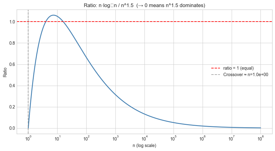
n·log n is larger than n^1.5 until approximately n = 1.00e+00
For n > 1.00e+00: n^1.5 = ω(n log n)
# --- Experiment 3: Practical threshold — when does algorithm complexity matter? ---
# Hypothesis: For n > some threshold, the growth rate determines feasibility
# regardless of hardware speed.
# Change OPS_PER_SEC to see how much better hardware helps.

import numpy as np

OPS_PER_SEC = 1e12    # <-- modify this (1e9=laptop, 1e12=fast workstation, 1e15=cluster)
TIME_LIMIT_SEC = 1.0  # <-- modify this (try 3600 for one hour, 86400 for one day)

def max_n_for(complexity_fn, ops, time_limit, max_n=10000):
    """Find maximum n where complexity_fn(n) / ops <= time_limit."""
    for n in range(1, max_n + 1):
        try:
            if complexity_fn(n) / ops > time_limit:
                return n - 1
        except (OverflowError, ValueError):
            return n - 1
    return max_n

import math
complexities = [
    ('O(log n)',   lambda n: math.log2(max(n, 1))),
    ('O(n)',       lambda n: n),
    ('O(n log n)', lambda n: n * math.log2(max(n, 1))),
    ('O(n²)',      lambda n: n**2),
    ('O(n³)',      lambda n: n**3),
    ('O(2^n)',     lambda n: 2.0**n),
    ('O(n!)',      lambda n: float(math.factorial(n)) if n <= 20 else float('inf')),
]

print(f"Maximum feasible input size n (ops={OPS_PER_SEC:.0e}/s, time={TIME_LIMIT_SEC}s)")
print("-" * 50)
for name, fn in complexities:
    n_max = max_n_for(fn, OPS_PER_SEC, TIME_LIMIT_SEC)
    print(f"  {name:15s}: n_max ≈ {n_max}")
Maximum feasible input size n (ops=1e+12/s, time=1.0s)
--------------------------------------------------
O(log n) : n_max ≈ 10000
O(n) : n_max ≈ 10000
O(n log n) : n_max ≈ 10000
O(n²) : n_max ≈ 10000
O(n³) : n_max ≈ 10000
O(2^n) : n_max ≈ 39
O(n!) : n_max ≈ 14
7. Exercises
Easy 1. Rank these functions in order of growth (slowest to fastest): n³, 3^n, n!, n log n, √n, log(log n), n^0.01. Verify numerically for n = 100.
Easy 2. Prove (using the limit definition) that 5n² + 3n + 7 = Θ(n²). Identify the constants C₁, C₂, and n₀ such that C₁n² ≤ 5n² + 3n + 7 ≤ C₂n² for all n > n₀.
Medium 1. Plot n! and Stirling’s approximation on a log scale for n = 1..50. On the same plot, add 2^n and n^n. Verify the hierarchy 2^n < n! < n^n numerically.
Medium 2. You have two sorting algorithms: A runs in 5n log n operations; B runs in 0.001 n². For what value of n does B become slower than A? Solve analytically and verify numerically.
Hard. Prove that n^k = o(a^n) for any k > 0 and a > 1 using L’Hôpital’s rule (you may use the rule without formal proof: if lim f(n)/g(n) is ∞/∞, it equals lim f'(n)/g'(n)). How many applications of L’Hôpital does it take?
8. Mini Project: Empirical Complexity Measurement
# --- Mini Project: Recovering complexity from timing data ---
#
# Problem:
#   Given a black-box function, determine its asymptotic complexity
#   by measuring its runtime at different input sizes and fitting
#   a growth model.
#
# Method:
#   1. Time the function at input sizes n₁, n₂, ..., nₖ
#   2. Plot time vs n on log-log axes
#   3. The slope of the log-log line gives the exponent of the polynomial
#   4. If the log-log plot curves (not straight), suspect exponential or factorial

import numpy as np
import time
import matplotlib.pyplot as plt

plt.style.use('seaborn-v0_8-whitegrid')

# Three black-box algorithms (complexity hidden)
def algo_A(n):
    """Unknown complexity — just benchmark it."""
    total = 0
    for i in range(n):
        for j in range(n):
            total += i + j
    return total

def algo_B(n):
    """Unknown complexity."""
    arr = list(range(n))
    for _ in range(int(n * np.log2(max(n, 2)))):
        arr[n // 2] += 1
    return sum(arr)

def algo_C(n):
    """Unknown complexity."""
    total = 0
    for i in range(n):
        total += i
    return total


def measure_timing(algo, sizes, repeats=3):
    """Time an algorithm at multiple input sizes."""
    times = []
    for n in sizes:
        runs = []
        for _ in range(repeats):
            start = time.perf_counter()
            algo(n)
            runs.append(time.perf_counter() - start)
        times.append(min(runs))  # take minimum (less noise)
    return np.array(times)


sizes = [50, 100, 150, 200, 300, 400, 500]

print("Measuring timing...")
t_A = measure_timing(algo_A, sizes)
t_B = measure_timing(algo_B, sizes)
t_C = measure_timing(algo_C, sizes)
print("Done.")

# Fit log-log slope: log(t) = slope × log(n) + const → t = C × n^slope
def fit_complexity_exponent(n_arr, t_arr):
    slope, _ = np.polyfit(np.log(n_arr), np.log(t_arr), 1)
    return slope

n_arr = np.array(sizes)
exp_A = fit_complexity_exponent(n_arr, t_A)
exp_B = fit_complexity_exponent(n_arr, t_B)
exp_C = fit_complexity_exponent(n_arr, t_C)

fig, ax = plt.subplots(figsize=(9, 5))
ax.loglog(n_arr, t_A, 'o-', label=f'Algo A (estimated exponent ≈ {exp_A:.2f})', color='red')
ax.loglog(n_arr, t_B, 's-', label=f'Algo B (estimated exponent ≈ {exp_B:.2f})', color='blue')
ax.loglog(n_arr, t_C, '^-', label=f'Algo C (estimated exponent ≈ {exp_C:.2f})', color='green')
ax.set_title('Empirical Complexity Measurement (Log-Log Plot)')
ax.set_xlabel('Input size n (log scale)')
ax.set_ylabel('Time (s) (log scale)')
ax.legend()
plt.tight_layout()
plt.show()

print(f"\nEmpirical exponents:")
print(f"  Algo A: n^{exp_A:.2f}  → {'O(n²)?' if abs(exp_A-2)<0.3 else 'examine further'}")
print(f"  Algo B: n^{exp_B:.2f}  → {'O(n log n)?' if 1.0 < exp_B < 1.3 else 'examine further'}")
print(f"  Algo C: n^{exp_C:.2f}  → {'O(n)?' if abs(exp_C-1)<0.2 else 'examine further'}")
9. Chapter Summary & Connections
The growth hierarchy
O(1) < O(log n) < O(n) < O(n log n) < O(n²) < O(2ⁿ) < O(n!)is strict: every entry eventually dominates all entries to its left, regardless of constant factors.O, Ω, Θ notation provides the vocabulary to state growth comparisons precisely. The limit test
lim f/gidentifies the relationship cleanly.Stirling’s approximation
n! ≈ √(2πn)(n/e)^nshows that factorial growth has an exponent that itself grows — placing it above any fixed exponential.Empirical complexity measurement via log-log slope fitting is a practical tool for characterizing black-box algorithms.
Backward connection: This chapter synthesizes the growth behavior from ch042 (Exponential Growth), the scale intuition from ch044 (Logarithmic Scales), and the exponent arithmetic from ch041 (Exponents and Powers) into a single comparative framework.
Forward connections:
ch047 (Orders of Magnitude) applies this hierarchy to physical and computational scale — connecting growth rates to real measurements.
The asymptotic notation introduced here is used throughout Part VI (Linear Algebra) to analyze matrix multiplication cost —
O(n³)naive vsO(n^{2.37})for Strassen-type algorithms.The factorial count of permutations connects to ch253 (Probability Rules) —
n!is the number of ways to arrangenitems, the foundation of combinatorics.
Going deeper: Introduction to Algorithms (CLRS), Chapter 3 — the standard reference for asymptotic notation. The appendix contains the full proof that n^k = o(a^n) for a > 1.