Prerequisites: ch051 (What is a Function?), ch003 (Abstraction)
You will learn:
The precise correspondence between mathematical functions and Python functions
Pure functions vs impure functions, and why purity matters mathematically
Higher-order functions: map, filter, reduce as mathematical operations
Lambda calculus intuition: functions as the universal building block
Environment: Python 3.x, numpy, matplotlib
1. Concept
In ch051 we defined a function mathematically. Now we ask: what is the relationship between a mathematical function and a program function?
The correspondence is exact for pure functions.
A pure function in programming:
Takes inputs, returns output
No side effects (no printing, no file writing, no modifying global state)
Deterministic: same input → same output, always
This is literally the definition of a mathematical function. A pure Python function def f(x): return x**2 is the function f(x) = x².
Where they diverge: Programming functions can be impure — they can read from files, use randomness, modify global state, print to screen. A mathematical function cannot. When a function takes a timestamp as input and returns it, it is pure. When it reads the current time and returns it, it is not.
Why this matters: Mathematical analysis tools (derivatives, limits, composition, inversion) work on pure functions. If your program function has side effects, you cannot apply mathematical reasoning to it.
2. Intuition & Mental Models
Physical analogy: A mathematical function is like a sealed black box — you feed in a number, it produces a number. No memory, no state, no history. A pure Python function is the same sealed box. An impure function is a box with a window to the outside — it can peek at the world and produce different outputs even for the same input.
Computational analogy: In functional programming languages (Haskell, Erlang), all functions are pure by default. This makes them behave exactly like mathematical functions. Python allows both, which is powerful but requires discipline.
Think of map(f, [1,2,3,4]) as applying f to each element of a set: {f(1), f(2), f(3), f(4)}. This is exactly the set-theoretic image of a set under a function — introduced in ch051.
Lambda calculus intuition: Every computable function can be expressed as a combination of input-output mappings. The lambda keyword in Python is a direct reference to this. lambda x: x**2 and def f(x): return x**2 define the same function — they are two syntactic representations of one mathematical object.
3. Visualization
# --- Visualization: Pure vs Impure Functions and their mathematical equivalents ---
import numpy as np
import matplotlib.pyplot as plt
plt.style.use('seaborn-v0_8-whitegrid')

# Demonstrating that pure functions produce consistent, plottable surfaces
# while impure functions do not.

# Pure function: same x → same y, always
def pure_f(x):
    return np.sin(x) * np.exp(-0.1 * x)

x = np.linspace(0, 10 * np.pi, 500)
y_pure = pure_f(x)

# Impure function: same x → different y (random noise added)
# This is NOT a mathematical function — it is non-deterministic.
def impure_f(x):
    return np.sin(x) * np.exp(-0.1 * x) + np.random.normal(0, 0.3)

# Call impure 3 times at same x — get 3 different "outputs"
y_impure_1 = np.array([impure_f(xi) for xi in x])
y_impure_2 = np.array([impure_f(xi) for xi in x])

fig, axes = plt.subplots(1, 2, figsize=(14, 5))

axes[0].plot(x, y_pure, color='steelblue', linewidth=1.5)
axes[0].set_title('Pure Function: f(x) = sin(x)·e^{-0.1x}\nSame input → always same output')
axes[0].set_xlabel('x')
axes[0].set_ylabel('f(x)')

axes[1].plot(x, y_impure_1, color='crimson', alpha=0.6, linewidth=1, label='Call 1')
axes[1].plot(x, y_impure_2, color='darkorange', alpha=0.6, linewidth=1, label='Call 2')
axes[1].set_title('Impure Function: adds random noise\nSame input → different outputs each call')
axes[1].set_xlabel('x')
axes[1].set_ylabel('f(x)')
axes[1].legend()

plt.tight_layout()
plt.show()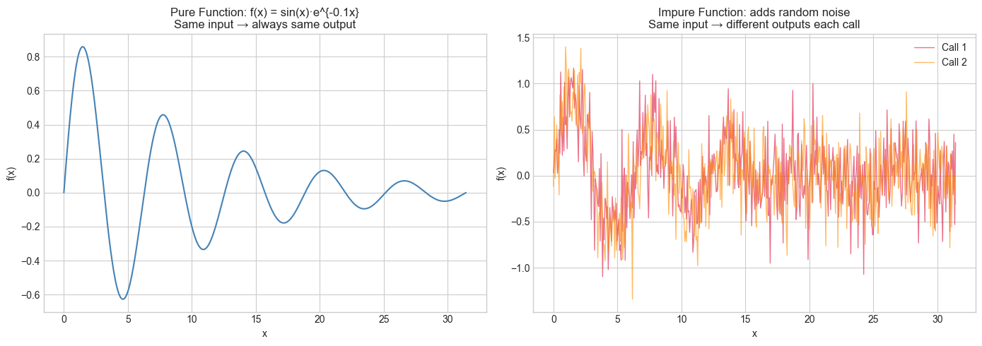
4. Mathematical Formulation
Function as a program — the lambda calculus view:
In lambda calculus, every function is written:
λx. [body]meaning: “a function that takes x and returns [body]”.
In Python: lambda x: body
Higher-order functions are functions that take other functions as input:
map(f, S)computes{f(x) : x ∈ S}— the image of set S under ffilter(p, S)computes{x ∈ S : p(x) is True}— subset where predicate holdsreduce(f, S)computesf(f(...f(x1, x2), x3)..., xn)— fold left
These are set operations expressed as programs.
# --- Mathematical Formulation: Higher-order functions as set operations ---
import numpy as np
from functools import reduce

# The input set S = {1, 2, 3, 4, 5, 6, 7, 8, 9, 10}
S = list(range(1, 11))

# map: apply f to every element
# Mathematical: { x² : x ∈ S }
squares = list(map(lambda x: x**2, S))
print("map (x²):", squares)

# filter: keep only elements satisfying a predicate
# Mathematical: { x ∈ S : x is even }
evens = list(filter(lambda x: x % 2 == 0, S))
print("filter (even):", evens)

# reduce: fold an operation over the set
# Mathematical: x1 + x2 + ... + xn = Σ xᵢ
total = reduce(lambda acc, x: acc + x, S, 0)
print("reduce (sum):", total)

# Composing: sum of squares of even numbers
# Mathematical: Σ { x² : x ∈ S, x even }
result = reduce(lambda acc, x: acc + x,
                map(lambda x: x**2,
                    filter(lambda x: x % 2 == 0, S)), 0)
print("Sum of squares of evens:", result)  # 4+16+36+64+100 = 220

# Verify:
print("Verify with numpy:", sum(x**2 for x in range(1,11) if x % 2 == 0))
map (x²): [1, 4, 9, 16, 25, 36, 49, 64, 81, 100]
filter (even): [2, 4, 6, 8, 10]
reduce (sum): 55
Sum of squares of evens: 220
Verify with numpy: 220
5. Python Implementation
# --- Implementation: Function utilities — memoization and profiling ---
import numpy as np
import time

def memoize(f):
    """
    Memoize a pure function: cache results so each input is only computed once.

    Mathematically valid ONLY for pure functions — since f(x) is always the same,
    we can safely cache it. For impure functions, memoization would give wrong results.

    Args:
        f: callable, a pure function
    Returns:
        callable: memoized version of f
    """
    cache = {}
    def memoized(x):
        if x not in cache:
            cache[x] = f(x)
        return cache[x]
    memoized.cache = cache  # expose for inspection
    return memoized

# Naive recursive Fibonacci — exponential time
def fib(n):
    """Fibonacci sequence: fib(n) = fib(n-1) + fib(n-2), fib(0)=0, fib(1)=1."""
    if n <= 1:
        return n
    return fib(n-1) + fib(n-2)

# Memoized version — polynomial time
@memoize
def fib_memo(n):
    """Memoized Fibonacci."""
    if n <= 1:
        return n
    return fib_memo(n-1) + fib_memo(n-2)

# Time comparison
N = 30

t0 = time.time()
result_naive = fib(N)
t_naive = time.time() - t0

t0 = time.time()
result_memo = fib_memo(N)
t_memo = time.time() - t0

print(f"fib({N}) = {result_naive}")
print(f"Naive time:    {t_naive:.4f}s")
print(f"Memoized time: {t_memo:.6f}s")
print(f"Speedup: {t_naive/max(t_memo, 1e-9):.1f}x")

# Memoization is sound BECAUSE fib is a pure function.
# The mathematical property (same input → same output) enables this optimization.
fib(30) = 832040
Naive time: 0.2916s
Memoized time: 0.000157s
Speedup: 1858.9x
6. Experiments
# --- Experiment 1: Function pipeline — composing transformations ---
# Hypothesis: Chaining pure functions produces a predictable composite transformation.
# Try changing: the order of the pipeline steps, or the functions themselves.

import numpy as np
import matplotlib.pyplot as plt
plt.style.use('seaborn-v0_8-whitegrid')

# Build a pipeline of transformations
pipeline = [
    ('shift_right', lambda x: x - 2),       # x → x - 2
    ('square',      lambda x: x**2),          # x → x²
    ('normalize',   lambda x: x / (x.max() + 1e-8)),  # x → x / max(x)
]

x = np.linspace(-5, 5, 300)
stages = [x]
labels = ['Input x']

current = x.copy()
for name, fn in pipeline:
    current = fn(current)
    stages.append(current.copy())
    labels.append(name)

fig, axes = plt.subplots(1, 4, figsize=(16, 4))
for ax, stage, label in zip(axes, stages, labels):
    ax.plot(x, stage, color='steelblue', linewidth=1.5)
    ax.set_title(label)
    ax.set_xlabel('Original x')
    ax.set_ylabel('Value')

plt.suptitle('Function Pipeline: Each step transforms the previous output', fontweight='bold')
plt.tight_layout()
plt.show()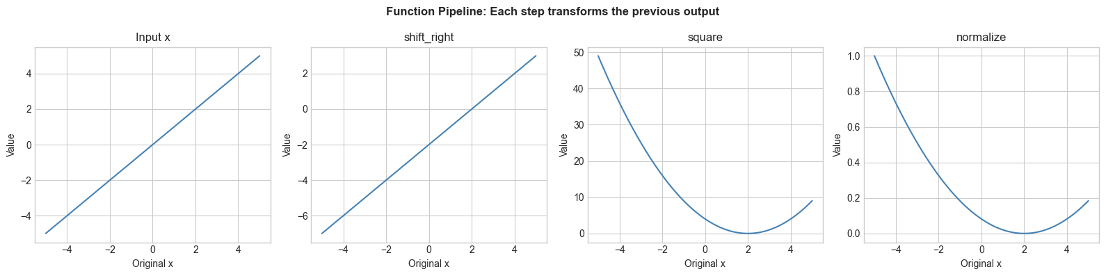
# --- Experiment 2: Purity test ---
# Hypothesis: Adding a global state variable to a function makes it impure.
# Try: run the pure and impure versions multiple times and compare outputs.

# IMPURE version — depends on external state
global_bias = 0.0

def impure_add(x):
    """NOT a mathematical function — reads external state."""
    global global_bias
    global_bias += 0.1  # mutates external state
    return x + global_bias

# PURE version
def pure_add(x, bias):
    """Mathematical function — all inputs explicit."""
    return x + bias

print("Calling impure_add(5) three times:")
print(impure_add(5))  # different each time!
print(impure_add(5))
print(impure_add(5))

print("\nCalling pure_add(5, 0.1) three times:")
print(pure_add(5, 0.1))  # same every time
print(pure_add(5, 0.1))
print(pure_add(5, 0.1))

# Lesson: to make an impure function pure, make all its dependencies explicit arguments.
Calling impure_add(5) three times:
5.1
5.2
5.3
Calling pure_add(5, 0.1) three times:
5.1
5.1
5.1
7. Exercises
Easy 1. Is random.randint(1, 6) a mathematical function? Why or why not? What change would make it one? (Expected: no; fix by adding a seed parameter)
Easy 2. Write a pipeline function compose(*fns) that takes any number of functions and returns a new function that applies them left-to-right. Test it with compose(lambda x: x+1, lambda x: x*2, lambda x: x-3) applied to 5. (Expected: a single callable)
Medium 1. Implement my_map(f, xs) without using the built-in map. Then implement it again using list comprehension. Show they produce identical results for f = lambda x: x**3 and xs = range(10). (Hint: iteration)
Medium 2. A function f is called idempotent if f(f(x)) = f(x) for all x. Write a test is_idempotent(f, test_values) and verify it holds for f = lambda x: abs(x), f = lambda x: x**2, and f = np.floor. Which ones are idempotent? (Hint: floor(floor(x)) = floor(x))
Hard. Implement a general memoize decorator that works for functions with multiple arguments (not just one). It should cache based on a tuple of all arguments. Then benchmark it on a recursive function that computes binomial coefficients C(n,k) = C(n-1,k-1) + C(n-1,k) and compare against the naive recursive version. (Challenge: extend to handle numpy arrays as arguments using a hash)
8. Mini Project
# --- Mini Project: Functional Data Processing Pipeline ---
# Problem: Process a dataset of temperature readings through a series of
#          pure transformation functions: clean → scale → smooth → analyze.
# Dataset: Simulated hourly temperature data with noise and outliers.
# Task: Build a composable, pure-function pipeline and report key statistics.

import numpy as np
import matplotlib.pyplot as plt
plt.style.use('seaborn-v0_8-whitegrid')

# --- Generate dataset ---
np.random.seed(7)
N_HOURS = 168  # one week
true_temp = 20 + 8 * np.sin(2 * np.pi * np.arange(N_HOURS) / 24)  # daily cycle
noisy_temp = true_temp + np.random.normal(0, 1.5, N_HOURS)
# Add outliers
outlier_idx = np.random.choice(N_HOURS, 10, replace=False)
noisy_temp[outlier_idx] += np.random.choice([-15, 15], 10)

# --- Pure transformation functions ---
def remove_outliers(x, z_threshold=2.5):
    """Replace values > z_threshold std deviations from mean with interpolated values."""
    mean, std = x.mean(), x.std()
    cleaned = x.copy()
    mask = np.abs(x - mean) > z_threshold * std
    # Replace outliers with linear interpolation
    indices = np.arange(len(x))
    cleaned[mask] = np.interp(indices[mask], indices[~mask], x[~mask])
    return cleaned

def celsius_to_fahrenheit(x):
    """Linear scaling: C → F."""
    return x * 9/5 + 32

def moving_average(x, window=5):
    """Smooth with a centered moving average."""
    return np.convolve(x, np.ones(window)/window, mode='same')

# TODO: Build the pipeline and visualize each stage
stages = {
    'Raw (°C)':        noisy_temp,
    'Cleaned (°C)':    remove_outliers(noisy_temp),
    'Fahrenheit':      celsius_to_fahrenheit(remove_outliers(noisy_temp)),
    'Smoothed (°F)':   moving_average(celsius_to_fahrenheit(remove_outliers(noisy_temp)))
}

fig, axes = plt.subplots(2, 2, figsize=(14, 8))
hours = np.arange(N_HOURS)
colors = ['crimson', 'darkorange', 'steelblue', 'darkgreen']

for ax, (label, data), color in zip(axes.flat, stages.items(), colors):
    ax.plot(hours, data, color=color, linewidth=1.2)
    ax.set_title(label)
    ax.set_xlabel('Hour')
    ax.set_ylabel('Temperature')

plt.suptitle('Pure Function Pipeline: Temperature Data Processing', fontsize=13, fontweight='bold')
plt.tight_layout()
plt.show()
9. Chapter Summary & Connections
What we covered:
Pure functions in Python correspond exactly to mathematical functions
Purity means: no side effects, deterministic, all dependencies as explicit arguments
Higher-order functions (map, filter, reduce) are set operations expressed as programs
Memoization is only correct for pure functions — it exploits the determinism guarantee
Backward connection: This extends ch051 — now we know not just what a function is, but how to implement one correctly in code.
Forward connections:
In ch054 (Function Composition), we will formalize the
composepattern and see it as a mathematical operation in its own rightIn ch075 (Recursion and Mathematical Functions), we will see recursive functions as a direct encoding of mathematical induction
This concept reappears in ch207 (Automatic Differentiation) where pure functions are a prerequisite for correct gradient computation