Prerequisites: ch051 (What is a Function?), ch026 (Real Numbers), ch038 (Floating-Point)
You will learn:
Precise definitions of domain, codomain, and range (image)
Natural domain vs restricted domain
How domain restrictions arise in computation (division, square roots, logs)
How to determine range analytically and computationally
Environment: Python 3.x, numpy, matplotlib
1. Concept
The domain of a function f : A → B is the set A — all valid inputs.
The codomain is the set B — all possible outputs by declaration.
The range (or image) is {f(x) : x ∈ A} — all outputs that are actually produced.
The range is always a subset of the codomain, but they need not be equal.
Natural domain: the largest set on which a formula is defined without causing mathematical errors. For f(x) = 1/x, the natural domain is all real numbers except 0. For f(x) = √x, it is x ≥ 0.
Restricted domain: a subset of the natural domain, chosen deliberately. We might restrict f(x) = x² to x ≥ 0 to make it invertible.
Common misconception: Codomain and range are the same thing. They are not. f(x) = x² declared as f : ℝ → ℝ has codomain ℝ but range [0, ∞). The range is determined by the formula; the codomain is declared by the programmer or mathematician.
Why it matters in programming: Every time you call np.log(x) with x ≤ 0, or 1/x with x = 0, you have violated the domain. NumPy returns nan or inf instead of raising an error — a silent failure. Knowing the domain of every function you use prevents this.
2. Intuition & Mental Models
Physical analogy: A vending machine (from ch051) has a domain: the set of valid codes. If you enter an invalid code, nothing happens (or an error message appears). The domain is the set of codes that trigger a response. The range is the set of snacks that are actually available — a subset of everything in the world.
Computational analogy: In programming, the domain of a function is its valid input contract. The range is its valid output contract. When you write type annotations like def f(x: float) -> float, you are declaring the codomain (float), not the range.
Think of a function as a machine with a red zone (undefined inputs) and a green zone (valid inputs). The domain is the green zone. For log(x), the red zone is x ≤ 0. For sqrt(x) over the reals, the red zone is x < 0.
3. Visualization
# --- Visualization: Domain restrictions for common functions ---
import numpy as np
import matplotlib.pyplot as plt
plt.style.use('seaborn-v0_8-whitegrid')

fig, axes = plt.subplots(2, 3, figsize=(16, 9))

functions = [
    # (name, domain_range, fn, domain_label, range_label)
    ('f(x) = 1/x',  np.concatenate([np.linspace(-3, -0.01, 200), np.linspace(0.01, 3, 200)]),
     lambda x: 1/x, 'x ≠ 0', 'y ≠ 0'),
    ('f(x) = √x',   np.linspace(0, 9, 400),
     np.sqrt, 'x ≥ 0', 'y ≥ 0'),
    ('f(x) = log(x)', np.linspace(0.01, 10, 400),
     np.log, 'x > 0', 'all reals'),
    ('f(x) = x²',   np.linspace(-3, 3, 400),
     lambda x: x**2, 'all reals', 'y ≥ 0'),
    ('f(x) = sin(x)', np.linspace(-2*np.pi, 2*np.pi, 400),
     np.sin, 'all reals', '[-1, 1]'),
    ('f(x) = arcsin(x)', np.linspace(-1, 1, 400),
     np.arcsin, '[-1, 1]', '[-π/2, π/2]'),
]

for ax, (name, x_vals, fn, dom, rng) in zip(axes.flat, functions):
    y_vals = fn(x_vals)
    ax.plot(x_vals, y_vals, color='steelblue', linewidth=2)
    ax.set_title(f'{name}\nDomain: {dom}  |  Range: {rng}', fontsize=9)
    ax.set_xlabel('x')
    ax.set_ylabel('f(x)')
    # Shade the valid domain
    ax.axhline(0, color='black', linewidth=0.5)
    ax.axvline(0, color='black', linewidth=0.5)

plt.suptitle('Domain and Range for Common Functions', fontsize=13, fontweight='bold')
plt.tight_layout()
plt.show()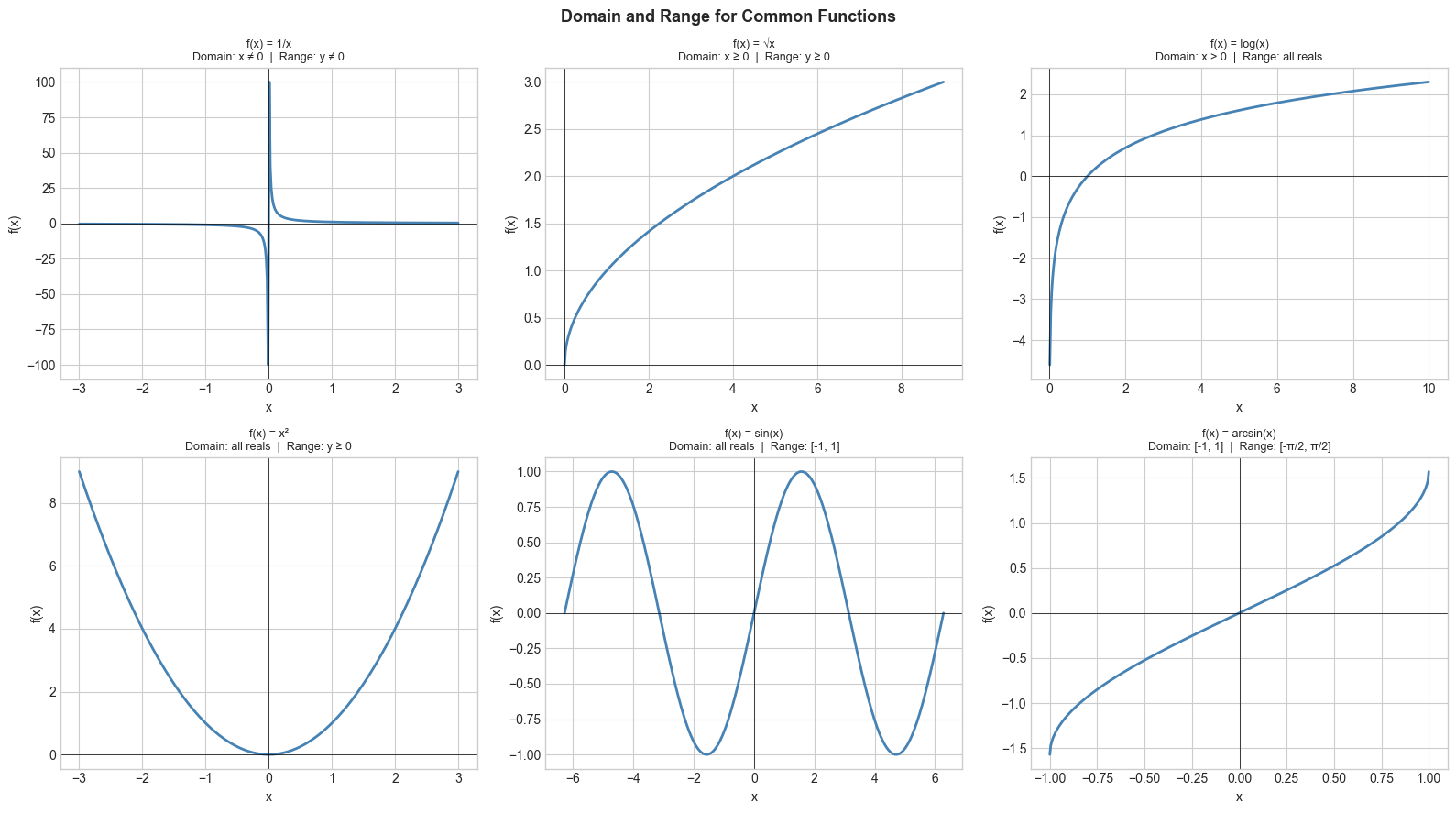
4. Mathematical Formulation
For a function f : A → B:
Domain: dom(f) = A
Codomain: cod(f) = B
Range (image): im(f) = {f(x) : x ∈ A} ⊆ B
Surjective (onto): im(f) = B — every element of B is hit Injective (one-to-one): f(x₁) = f(x₂) implies x₁ = x₂ — no two inputs share an output Bijective: both injective and surjective — perfect pairing between A and B
These properties determine whether a function has an inverse (ch055).
# --- Mathematical Formulation: Determining range numerically ---
import numpy as np

def numerical_range(f, domain_start, domain_end, n_samples=10000):
    """
    Estimate the range of function f over a domain interval.
    Uses dense sampling — gives approximate min and max of the range.

    Args:
        f: callable, function from reals to reals
        domain_start, domain_end: float, domain interval
        n_samples: int, number of sample points
    Returns:
        (min_val, max_val): approximate range bounds
    """
    x = np.linspace(domain_start, domain_end, n_samples)
    y = f(x)
    # Filter out nan/inf (undefined points)
    y_valid = y[np.isfinite(y)]
    if len(y_valid) == 0:
        return None, None
    return y_valid.min(), y_valid.max()

# Test on known functions
test_cases = [
    ('x²  on [-3, 3]',  lambda x: x**2,   -3, 3),
    ('sin(x) on [-2π, 2π]', np.sin,       -2*np.pi, 2*np.pi),
    ('log(x) on [0.01, 10]', np.log,       0.01, 10),
    ('1/x on [0.1, 5]', lambda x: 1/x,    0.1, 5),
]

for name, f, a, b in test_cases:
    lo, hi = numerical_range(f, a, b)
    print(f"Range of {name}: [{lo:.4f}, {hi:.4f}]")
Range of x² on [-3, 3]: [0.0000, 9.0000]
Range of sin(x) on [-2π, 2π]: [-1.0000, 1.0000]
Range of log(x) on [0.01, 10]: [-4.6052, 2.3026]
Range of 1/x on [0.1, 5]: [0.2000, 10.0000]
5. Python Implementation
# --- Implementation: Domain-aware function wrapper ---
import numpy as np

class DomainAwareFunction:
    """
    Wraps a mathematical function with explicit domain checking.
    Raises ValueError for inputs outside the domain.
    Provides a safe vectorized apply method.
    """

    def __init__(self, f, domain_predicate, name='f', domain_description='unknown'):
        """
        Args:
            f: callable, the underlying function
            domain_predicate: callable, returns True if x is in domain
            name: str, function name for error messages
            domain_description: str, human-readable domain description
        """
        self.f = f
        self.domain_predicate = domain_predicate
        self.name = name
        self.domain_description = domain_description

    def __call__(self, x):
        """Apply function, raising ValueError if x is outside domain."""
        x = np.asarray(x, dtype=float)
        valid = self.domain_predicate(x)
        if not np.all(valid):
            bad = x[~valid] if x.ndim > 0 else x
            raise ValueError(
                f"{self.name}: input {bad} outside domain ({self.domain_description})"
            )
        return self.f(x)

    def safe_apply(self, x, fill_value=np.nan):
        """Apply function, returning fill_value for out-of-domain inputs."""
        x = np.asarray(x, dtype=float)
        result = np.full_like(x, fill_value)
        valid = self.domain_predicate(x)
        result[valid] = self.f(x[valid])
        return result

# Create domain-aware versions of common functions
sqrt_safe = DomainAwareFunction(
    np.sqrt, lambda x: x >= 0, name='sqrt', domain_description='x >= 0'
)
log_safe = DomainAwareFunction(
    np.log, lambda x: x > 0, name='log', domain_description='x > 0'
)

# Demonstrate safe_apply with mixed valid/invalid inputs
test_inputs = np.array([-4, -1, 0, 1, 4, 9, 16])

print("Input:", test_inputs)
print("sqrt_safe:", sqrt_safe.safe_apply(test_inputs))   # nan for negatives
print("log_safe: ", log_safe.safe_apply(test_inputs))    # nan for non-positives
Input: [-4 -1 0 1 4 9 16]
sqrt_safe: [nan nan 0. 1. 2. 3. 4.]
log_safe: [ nan nan nan 0. 1.38629436 2.19722458
2.77258872]
6. Experiments
# --- Experiment 1: What happens when you violate a domain? ---
# Hypothesis: NumPy silently handles domain violations with nan/inf rather than erroring.
# Try: change which function and which values you test.
import numpy as np

print("Domain violations and NumPy's responses:")
print(f"  log(0)    = {np.log(0)}")
print(f"  log(-1)   = {np.log(-1)}")
print(f"  sqrt(-1)  = {np.sqrt(-1)}")
print(f"  1/0       = {1.0/0.0 if False else 'ZeroDivisionError — use np.float64'}")
print(f"  np.float64(1)/np.float64(0) = {np.float64(1)/np.float64(0)}")
print(f"  arcsin(2) = {np.arcsin(2)}")

# The silent nan/inf is DANGEROUS in ML — it propagates through all downstream ops
x = np.array([1.0, 0.0, -1.0, 4.0])
result = np.log(x)  # produces nan for non-positive values
print("\nlog([1, 0, -1, 4]) =", result)
print("sum =>", np.sum(result))  # NaN poisons everything!
print("\nLesson: always validate domain BEFORE applying the function.")
Domain violations and NumPy's responses:
log(0) = -inf
log(-1) = nan
sqrt(-1) = nan
1/0 = ZeroDivisionError — use np.float64
np.float64(1)/np.float64(0) = inf
arcsin(2) = nan
log([1, 0, -1, 4]) = [0. -inf nan 1.38629436]
sum => nan
Lesson: always validate domain BEFORE applying the function.
C:\Users\user\AppData\Local\Temp\ipykernel_9356\438985284.py:7: RuntimeWarning: divide by zero encountered in log
  print(f"  log(0)    = {np.log(0)}")
C:\Users\user\AppData\Local\Temp\ipykernel_9356\438985284.py:8: RuntimeWarning: invalid value encountered in log
  print(f"  log(-1)   = {np.log(-1)}")
C:\Users\user\AppData\Local\Temp\ipykernel_9356\438985284.py:9: RuntimeWarning: invalid value encountered in sqrt
  print(f"  sqrt(-1)  = {np.sqrt(-1)}")
C:\Users\user\AppData\Local\Temp\ipykernel_9356\438985284.py:11: RuntimeWarning: divide by zero encountered in scalar divide
  print(f"  np.float64(1)/np.float64(0) = {np.float64(1)/np.float64(0)}")
C:\Users\user\AppData\Local\Temp\ipykernel_9356\438985284.py:12: RuntimeWarning: invalid value encountered in arcsin
  print(f"  arcsin(2) = {np.arcsin(2)}")
C:\Users\user\AppData\Local\Temp\ipykernel_9356\438985284.py:16: RuntimeWarning: divide by zero encountered in log
  result = np.log(x)  # produces nan for non-positive values
C:\Users\user\AppData\Local\Temp\ipykernel_9356\438985284.py:16: RuntimeWarning: invalid value encountered in log
  result = np.log(x)  # produces nan for non-positive values
# --- Experiment 2: Injective, surjective, bijective ---
# Hypothesis: We can test these properties numerically for functions on finite sets.
# Try: change the function and the domain size.

import numpy as np

DOMAIN = list(range(1, 8))  # {1, 2, 3, 4, 5, 6, 7}  # <-- try changing this

def test_properties(f, domain, codomain=None):
    """Test injective and surjective properties numerically."""
    outputs = [f(x) for x in domain]

    # Injective: all outputs are distinct
    injective = len(outputs) == len(set(outputs))

    # Surjective: only testable if codomain is known
    surjective = None
    if codomain is not None:
        surjective = set(outputs) == set(codomain)

    return injective, surjective, outputs

# Test several functions
tests = [
    ('x → x² mod 7',  lambda x: (x**2) % 7, None),
    ('x → x mod 7',   lambda x: x % 7,      list(range(7))),
    ('x → 2x mod 7',  lambda x: (2*x) % 7,  list(range(7))),
    ('x → 3x mod 7',  lambda x: (3*x) % 7,  list(range(7))),
]

for name, f, cod in tests:
    inj, surj, out = test_properties(f, DOMAIN, cod)
    print(f"{name}:")
    print(f"  Outputs: {out}")
    print(f"  Injective: {inj}  |  Surjective: {surj}")
x → x² mod 7:
Outputs: [1, 4, 2, 2, 4, 1, 0]
Injective: False | Surjective: None
x → x mod 7:
Outputs: [1, 2, 3, 4, 5, 6, 0]
Injective: True | Surjective: True
x → 2x mod 7:
Outputs: [2, 4, 6, 1, 3, 5, 0]
Injective: True | Surjective: True
x → 3x mod 7:
Outputs: [3, 6, 2, 5, 1, 4, 0]
Injective: True | Surjective: True
7. Exercises
Easy 1. State the natural domain of each: (a) f(x) = (x-3)/(x²-9) (b) f(x) = log(log(x)) (c) f(x) = √(4-x²). (Expected: (a) x≠3 and x≠-3, (b) x>1, (c) -2≤x≤2)
Easy 2. For f(x) = x² with domain restricted to [0, 5], what is the range? Verify computationally by generating 10000 uniform random samples in [0,5] and finding the min/max of f(x). (Expected: [0, 25])
Medium 1. Write a function find_domain_intervals(f, x_min, x_max, n=10000) that samples f over [x_min, x_max] and returns a list of contiguous intervals where f is defined (i.e., produces finite values). Test on f(x) = log(x² - 4). (Hint: find where output is finite, then group contiguous indices)
Medium 2. The function f(x) = x² is not injective over ℝ, but becomes injective if restricted to [0, ∞). Write a function is_injective_on(f, domain_array, tolerance=1e-9) and verify this claim. (Hint: round values to handle floating point)
Hard. For f(x) = sin(x) on [-π/2, π/2], demonstrate numerically that f is both injective and surjective onto [-1, 1] (i.e., bijective). Then show that on [-π, π], f is surjective but not injective. Prove the non-injectivity by finding two distinct x values with the same f(x) value. (Challenge: what is the minimum domain extension needed to break injectivity?)
8. Mini Project
# --- Mini Project: Domain Boundary Detector ---
# Problem: Many ML preprocessing functions have hidden domain restrictions.
#          Build a tool that automatically detects where a function fails
#          and visualizes the valid and invalid regions.
# Dataset: Dense sample grid over a range containing edge cases.
# Task: For each test function, detect valid/invalid regions and plot them.

import numpy as np
import matplotlib.pyplot as plt
plt.style.use('seaborn-v0_8-whitegrid')

def detect_domain(f, x_min, x_max, n=5000):
    """
    Detect valid (finite) and invalid (nan/inf) input regions.
    Returns x_valid, y_valid, x_invalid.
    """
    x = np.linspace(x_min, x_max, n)
    with np.errstate(divide='ignore', invalid='ignore'):
        y = f(x)
    finite_mask = np.isfinite(y)
    return x[finite_mask], y[finite_mask], x[~finite_mask]

# Test on functions with interesting domain structures
funcs = [
    ('log(x² - 1)',  lambda x: np.log(x**2 - 1),  -3, 3),
    ('sqrt(sin(x))', lambda x: np.sqrt(np.sin(x)), -2*np.pi, 2*np.pi),
    ('1/(x²-3x+2)', lambda x: 1/(x**2 - 3*x + 2), -1, 4),
    ('arcsin(x/2)', lambda x: np.arcsin(x/2),      -3, 3),
]

fig, axes = plt.subplots(2, 2, figsize=(14, 8))

for ax, (name, f, a, b) in zip(axes.flat, funcs):
    xv, yv, xi = detect_domain(f, a, b)
    ax.plot(xv, yv, color='steelblue', linewidth=1.5, label='Defined')
    ax.scatter(xi, np.zeros_like(xi), color='crimson', s=2, alpha=0.3, label='Undefined')
    ax.axhline(0, color='black', linewidth=0.5)
    ax.set_title(f'f(x) = {name}')
    ax.set_xlabel('x')
    ax.set_ylabel('f(x)')
    ax.legend(fontsize=8)

plt.suptitle('Domain Boundary Detection', fontsize=13, fontweight='bold')
plt.tight_layout()
plt.show()
9. Chapter Summary & Connections
What we covered:
Domain = valid inputs; Codomain = declared output set; Range = actual outputs produced
Natural domain is determined by mathematical constraints (no division by zero, no log of negatives)
NumPy silently produces nan/inf for domain violations — always validate inputs
Injective (one-to-one) and surjective (onto) describe the input-output coverage properties
Backward connection: This makes precise what ch051 left vague — a function needs not just a rule but a set of valid inputs.
Forward connections:
In ch055 (Inverse Functions), we will see that injectivity is exactly the condition needed for an inverse to exist
Domain restrictions reappear in ch073 (Error and Residuals) — a model’s domain must cover all data points
In ch241 (Probability), sample spaces are the domain of probability functions — same concept, probabilistic setting