Prerequisites: ch051–055 (Function foundations)
You will learn:
Use matplotlib to visualize any function on a given domain
Compare multiple functions in the same plot
Identify key features: zeros, extrema, asymptotes visually
Build a reusable function plotter
Environment: Python 3.x, numpy, matplotlib
1. Concept
Visualization is not decoration — it is the fastest way to build intuition about a function’s behavior. Before computing anything analytically, plot it. The shape of a function reveals its zeros, monotonicity, asymptotes, growth rate, and periodicity at a glance.
A well-made function plot answers: where is f(x) = 0? Where is f increasing? Does it blow up? Does it repeat? These questions take pages of algebra but seconds of visual inspection.
2. Intuition & Mental Models
Physical analogy: A map is a visualization of a geographic function. The terrain shape is immediately obvious from contour lines — it would take hours to understand from a table of coordinates.
Computational analogy: A debugger’s watch variable is like reading a function table. A plot is like running a profiler — you see the whole picture at once.
Recall from ch008 (Visualization as a Learning Tool): the purpose of a plot is to reveal structure, not just to display data. Every axis label, grid line, and color choice is a communication decision.
3. Visualization
# --- Visualization: Multi-panel function explorer ---
import numpy as np
import matplotlib.pyplot as plt
plt.style.use('seaborn-v0_8-whitegrid')

def plot_function(f, x_min, x_max, ax, label, color='steelblue', n=1000):
    """Plot a function with zeros and extrema annotated."""
    x = np.linspace(x_min, x_max, n)
    y = f(x)
    ax.plot(x, y, color=color, linewidth=2, label=label)
    ax.axhline(0, color='black', linewidth=0.5)
    ax.axvline(0, color='black', linewidth=0.5)
    ax.set_xlabel('x')
    ax.set_ylabel('f(x)')
    ax.legend()

funcs = [
    (lambda x: x**3 - 3*x, -2.5, 2.5, 'x³ - 3x (cubic)'),
    (lambda x: np.sin(x) / x if True else None, 0.1, 4*np.pi, 'sin(x)/x (sinc-like)'),
    (lambda x: np.exp(-x**2), -3, 3, 'e^(-x²) (Gaussian)'),
    (lambda x: 1/(1 + x**2), -5, 5, '1/(1+x²) (Cauchy)'),
]

fig, axes = plt.subplots(2, 2, figsize=(12, 8))
colors = ['steelblue', 'crimson', 'darkgreen', 'darkorange']

for ax, (f, a, b, label), color in zip(axes.flat, funcs, colors):
    x = np.linspace(a, b, 1000)
    with np.errstate(invalid='ignore', divide='ignore'):
        y = f(x)
    ax.plot(x, np.where(np.isfinite(y), y, np.nan), color=color, linewidth=2)
    ax.axhline(0, color='black', linewidth=0.5)
    ax.set_title(label)
    ax.set_xlabel('x')
    ax.set_ylabel('f(x)')

plt.suptitle('Common Function Shapes — Key Patterns to Recognize', fontsize=13, fontweight='bold')
plt.tight_layout()
plt.show()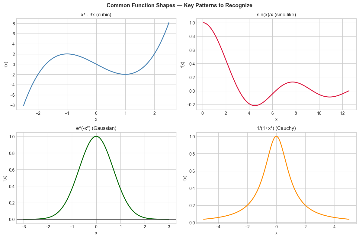
4. Mathematical Formulation
Key visual features to identify:
Zeros: where f(x) = 0 — the x-intercepts
Extrema: local maxima and minima
Asymptotes: vertical (where f→∞), horizontal (limiting value)
Monotonicity: where f is increasing vs decreasing
Symmetry: even (f(-x)=f(x)), odd (f(-x)=-f(x)), or neither
# --- Function feature detection ---
import numpy as np

def detect_zeros(f, x_min, x_max, n=10000, tol=0.01):
    """Find approximate zero crossings of f."""
    x = np.linspace(x_min, x_max, n)
    y = f(x)
    sign_changes = np.where(np.diff(np.sign(y)))[0]
    return x[sign_changes]

def detect_extrema(f, x_min, x_max, n=1000):
    """Find approximate local extrema using derivative sign changes."""
    x = np.linspace(x_min, x_max, n)
    y = f(x)
    dy = np.diff(y)
    sign_changes = np.where(np.diff(np.sign(dy)))[0]
    return x[sign_changes + 1], y[sign_changes + 1]

# Test on f(x) = x^3 - 3x
f = lambda x: x**3 - 3*x
zeros = detect_zeros(f, -3, 3)
ex_x, ex_y = detect_extrema(f, -3, 3)

print(f"Approximate zeros of x³-3x: {zeros.round(2)}")
print(f"Expected: x ≈ -1.73, 0, 1.73")
print(f"Approximate extrema: x={ex_x.round(2)}, f(x)={ex_y.round(2)}")
print(f"Expected: local max at x≈-1, local min at x≈1")
Approximate zeros of x³-3x: [-1.73 -0. 1.73]
Expected: x ≈ -1.73, 0, 1.73
Approximate extrema: x=[-1. 1.], f(x)=[ 2. -2.]
Expected: local max at x≈-1, local min at x≈1
5. Python Implementation
# --- Mini Project: Reusable function plotter with feature annotation ---
import numpy as np
import matplotlib.pyplot as plt
plt.style.use('seaborn-v0_8-whitegrid')

class FunctionPlotter:
    """Interactive-style plotter with auto annotation."""

    def __init__(self, f, x_min, x_max, name='f(x)', n=2000):
        self.f = f
        self.x_min = x_min
        self.x_max = x_max
        self.name = name
        self.n = n
        self.x = np.linspace(x_min, x_max, n)
        with np.errstate(invalid='ignore', divide='ignore'):
            self.y = f(self.x)

    def plot(self, ax=None, annotate=True):
        if ax is None:
            fig, ax = plt.subplots(figsize=(10, 5))

        ax.plot(self.x, self.y, linewidth=2, label=self.name)
        ax.axhline(0, color='black', linewidth=0.5)
        ax.axvline(0, color='black', linewidth=0.5)

        if annotate:
            # Mark zeros
            sign = np.sign(self.y)
            sign_changes = np.where(np.diff(sign) != 0)[0]
            for idx in sign_changes:
                ax.plot(self.x[idx], 0, 'ro', markersize=6, zorder=5)

            # Mark approximate extrema
            dy = np.diff(self.y)
            ext_idx = np.where(np.diff(np.sign(dy)) != 0)[0] + 1
            ax.plot(self.x[ext_idx], self.y[ext_idx], 'g^', markersize=6, zorder=5,
                    label='extrema')

        ax.set_title(f'{self.name} on [{self.x_min:.1f}, {self.x_max:.1f}]')
        ax.set_xlabel('x')
        ax.set_ylabel('f(x)')
        ax.legend()
        return ax

# Demo
plotter = FunctionPlotter(lambda x: np.sin(2*x) * np.exp(-0.2*x), 0, 3*np.pi, 'sin(2x)·e^{-0.2x}')
fig, ax = plt.subplots(figsize=(10, 5))
plotter.plot(ax)
plt.tight_layout()
plt.show()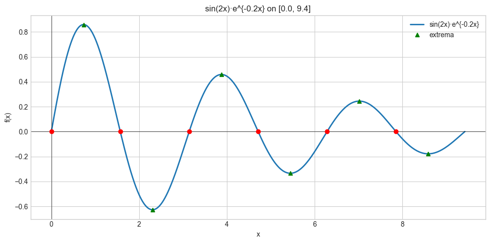
6. Experiments
Experiment 1: Plot f(x) = x^n for n = 1, 2, 3, 4, 5 on [-2, 2]. Observe how parity (even/odd n) determines symmetry. Try changing n to negative values.
Experiment 2: Compare f(x) = e^x and g(x) = x^10 on [0, 20]. Which dominates for large x? Try changing the exponent in g.
7. Exercises
Easy 1. Plot f(x) = (x-1)(x-2)(x-3) and identify its zeros from the graph. Verify analytically. (Expected: zeros at 1, 2, 3)
Easy 2. Write is_even(f, test_range) that checks if f(-x) ≈ f(x) for all x in test_range. Test on x², x³, cos(x), sin(x). (Expected: x², cos are even; x³, sin are odd)
Medium 1. Build a function annotated_plot(f, a, b) that plots f and automatically marks zero crossings with red circles and extrema with green triangles.
Medium 2. Plot the same function on three different x-ranges: [-0.1, 0.1], [-10, 10], [-1000, 1000] for f(x) = sin(x)/x. Describe how the visual impression changes.
Hard. Implement a function sniffer that automatically chooses a good x-range for plotting an arbitrary function: sample 100 points from [-100, 100], detect where the function is finite and varying, then zoom into the ‘interesting’ region.
9. Chapter Summary & Connections
Visualization reveals zeros, extrema, asymptotes, and monotonicity faster than algebra
matplotlibwith labeled axes and titles is the standard toolEven/odd symmetry is detectable visually and computationally
Feature detection (zeros, extrema) requires sign-change analysis
Forward connections:
In ch099 (Distance Between Points), we will visualize 2D functions as surface plots
Visualization tools built here scale directly to ch213 (Gradient Descent) where we plot loss landscapes
The extrema detection approach here is the visual precursor to derivatives in ch205