Prerequisites: ch051 (Functions), ch053 (Domain), ch056 (Visualization)
You will learn:
Define functions that use different rules on different parts of the domain
Implement piecewise functions efficiently with NumPy
Identify continuity and discontinuity at the boundary points
Connect to ReLU and other ML activation functions
Environment: Python 3.x, numpy, matplotlib
1. Concept
A piecewise function applies different formulas on different intervals of the domain.
General form: f(x) = { f₁(x) if x ∈ A₁; f₂(x) if x ∈ A₂; ... }
Examples:
|x| = { x if x ≥ 0; -x if x < 0 }
ReLU(x) = max(0, x) = { x if x ≥ 0; 0 if x < 0 }
Floor, ceiling, sign functions are piecewise
Continuity at boundaries: A piecewise function is continuous at a boundary point a if the left and right limits agree and equal f(a). If they disagree, there is a jump discontinuity.
Computational importance: Piecewise functions arise everywhere in ML:
ReLU and its variants are the most common neural activation functions
Decision trees partition the input space and apply constant functions per region
Clipping (gradient clipping, value clipping) is a piecewise operation
2. Intuition & Mental Models
Physical analogy: A tax bracket system. Different income ranges are taxed at different rates. The total tax function is piecewise linear — each bracket has its own slope.
Computational analogy: An if-else chain in code is exactly a piecewise function. if x > 0: return x else: return 0 is ReLU. The mathematical and computational representations are identical.
3. Visualization
# --- Visualization: Piecewise functions and continuity ---
import numpy as np
import matplotlib.pyplot as plt
plt.style.use('seaborn-v0_8-whitegrid')

x = np.linspace(-3, 3, 600)

def piecewise_demo(x):
    return np.piecewise(x,
        [x < -1, (x >= -1) & (x < 1), x >= 1],
        [lambda x: -x - 2,
         lambda x: x**2,
         lambda x: 2*x - 1])

def relu(x): return np.maximum(0, x)
def leaky_relu(x, alpha=0.1): return np.where(x >= 0, x, alpha * x)
def abs_val(x): return np.abs(x)

fig, axes = plt.subplots(1, 3, figsize=(15, 5))

axes[0].plot(x, piecewise_demo(x), color='steelblue', linewidth=2)
axes[0].axvline(-1, color='gray', linestyle='--', alpha=0.5)
axes[0].axvline(1, color='gray', linestyle='--', alpha=0.5)
axes[0].set_title('Custom piecewise function\n(continuous at boundaries)')
axes[0].set_xlabel('x'); axes[0].set_ylabel('f(x)')

for ax, (f, label, color) in zip([axes[1]]*3+[axes[2]]*2, [
    (relu, 'ReLU', 'steelblue'),
    (leaky_relu, 'Leaky ReLU (α=0.1)', 'crimson'),
    (abs_val, '|x|', 'darkgreen'),
]):
    pass  # handled below

axes[1].plot(x, relu(x), color='steelblue', linewidth=2, label='ReLU')
axes[1].plot(x, leaky_relu(x), color='crimson', linewidth=2, linestyle='--', label='Leaky ReLU')
axes[1].set_title('ML Activation Functions')
axes[1].set_xlabel('x'); axes[1].set_ylabel('f(x)')
axes[1].legend()

axes[2].plot(x, abs_val(x), color='darkgreen', linewidth=2, label='|x|')
axes[2].plot(x, np.where(x >= 0, 1, -1), color='darkorange', linewidth=2, label='sign(x)')
axes[2].set_title('Absolute Value and Sign')
axes[2].set_xlabel('x'); axes[2].set_ylabel('f(x)')
axes[2].legend()

plt.suptitle('Piecewise Functions: Structure and Continuity', fontsize=13, fontweight='bold')
plt.tight_layout()
plt.show()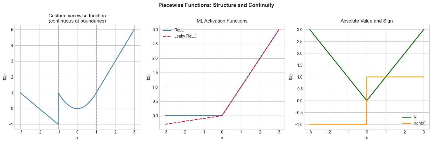
4. Mathematical Formulation
Continuity test at x = a: lim_{x→a⁻} f(x) = lim_{x→a⁺} f(x) = f(a)
If the left and right limits differ: jump discontinuity. If they agree but ≠ f(a): removable discontinuity.
np.piecewise(x, conditions, functions) is the vectorized implementation.
# --- Implementation: Piecewise function with continuity check ---
import numpy as np

def piecewise_fn(x):
    """Example piecewise function: linear-quadratic-linear."""
    x = np.asarray(x, dtype=float)
    return np.piecewise(x,
        [x < -1, (x >= -1) & (x < 1), x >= 1],
        [lambda x: -x, lambda x: x**2, lambda x: x])

def check_continuity(f, boundary, eps=1e-8):
    """Numerically check continuity at a boundary point."""
    left_limit = f(boundary - eps)
    right_limit = f(boundary + eps)
    value = f(boundary)
    continuous = (np.abs(left_limit - right_limit) < 1e-6 and
                  np.abs(value - right_limit) < 1e-6)
    return continuous, left_limit, right_limit, value

for boundary in [-1, 0, 1]:
    cont, ll, rl, val = check_continuity(piecewise_fn, boundary)
    print(f"At x={boundary}: left={ll:.4f}, right={rl:.4f}, f({boundary})={val:.4f} => {'CONTINUOUS' if cont else 'DISCONTINUOUS'}")
At x=-1: left=1.0000, right=1.0000, f(-1)=1.0000 => CONTINUOUS
At x=0: left=0.0000, right=0.0000, f(0)=0.0000 => CONTINUOUS
At x=1: left=1.0000, right=1.0000, f(1)=1.0000 => CONTINUOUS
6. Experiments
Experiment 1: Modify piecewise_demo to create a discontinuity at x=1. Change the right piece to 2*x - 2 instead of 2*x - 1. Observe the jump visually.
Experiment 2: Compare ReLU and Leaky ReLU at x=-1, -0.1, 0. What happens to very negative inputs under standard ReLU? (This is the ‘dying ReLU’ problem in deep learning.)
7. Exercises
Easy 1. Write a piecewise function for the absolute value |x| without using abs or np.abs. Test on [-3, -1, 0, 1, 3].
Easy 2. Implement the tax function: 10% on first 20k-80k. Test on incomes [0, 10000, 30000, 100000].
Medium 1. Implement the Huber loss: L(x) = { x²/2 if |x|≤δ; δ(|x| - δ/2) if |x|>δ }. Plot for δ=1 and compare to |x|. Where is it smooth?
Medium 2. Implement smooth_piecewise(f1, f2, boundary, width) that smoothly blends f1 and f2 near the boundary using a sigmoid transition.
Hard. The sign function sign(x) is discontinuous at x=0. Implement a smooth approximation sign_smooth(x, k) = tanh(kx) that converges to sign(x) as k→∞. Plot for k=1, 5, 20, 100.
9. Chapter Summary & Connections
Piecewise functions use different rules on different intervals
np.piecewiseandnp.whereare the NumPy idioms for vectorized piecewise computationContinuity at boundaries: check left and right limits numerically
ReLU, Leaky ReLU, step functions are all piecewise — the foundations of modern ML activations
Forward connections:
ch063 (Step Functions) deepens the discontinuity analysis
ch065 (Activation Functions in ML) catalogs the full family of ML activations
Piecewise linear functions form decision tree models in ch293 (Classification)