Prerequisites: Part III (Functions). Basic Python and numpy.
Outcomes: Connect mathematical geometry to programming primitives; Represent geometric objects as data structures; Understand why geometry matters for ML and graphics
Why Geometry for Programmers
Geometry is the mathematics of space and shape. For programmers, it appears in:
Computer graphics: every pixel rendered requires geometric computation
Machine learning: data lives in high-dimensional space; distance, angles, projections are central
Game development: collision detection, physics, pathfinding
Robotics: coordinate transforms, sensor geometry, motion planning
GIS and mapping: distances on spheres, projections, spatial queries
In this Part, we work in 2D. The ideas extend to 3D and beyond. The key insight: geometric objects are data structures; geometric operations are functions.
Representing Geometry as Data
| Object | Representation |
|---|---|
| Point | (x, y) — a tuple or length-2 array |
| Line segment | (p1, p2) — two points |
| Line (infinite) | (a, b, c) — coefficients of ax + by + c = 0 |
| Circle | (center, radius) — point + scalar |
| Polygon | list of vertices (ordered) |
| Vector | (dx, dy) — displacement, not position |
In code, numpy arrays are the universal container. A set of N points is an (N, 2) array. A transformation is a (2, 2) or (3, 3) matrix (ch114).
(Points introduced in ch092; transformations in ch108–114. This is the data-structure preview.)
# --- Geometry data structures ---
import numpy as np
import matplotlib.pyplot as plt
plt.style.use('seaborn-v0_8-whitegrid')

# Represent a triangle as a (3, 2) array
triangle = np.array([[0, 0], [4, 0], [2, 3]], dtype=float)

# Represent a circle as (center, radius)
circle = {'center': np.array([2.0, 1.0]), 'radius': 1.5}

# Represent a line as ax + by + c = 0
# Line y = 0.5x + 1  →  -0.5x + y - 1 = 0  →  (a=-0.5, b=1, c=-1)
line = {'a': -0.5, 'b': 1.0, 'c': -1.0}

# Plot all three
fig, ax = plt.subplots(figsize=(8, 7))

# Triangle
closed = np.vstack([triangle, triangle[0]])
ax.fill(triangle[:,0], triangle[:,1], alpha=0.2, color='steelblue')
ax.plot(closed[:,0], closed[:,1], 'steelblue', linewidth=2, label='Triangle')
for i, (x, y) in enumerate(triangle):
    ax.annotate(f'P{i}({x:.0f},{y:.0f})', (x, y), textcoords='offset points', xytext=(5,5), fontsize=9)

# Circle
theta = np.linspace(0, 2*np.pi, 100)
cx, cy, r = circle['center'][0], circle['center'][1], circle['radius']
ax.plot(cx + r*np.cos(theta), cy + r*np.sin(theta), 'crimson', linewidth=2, label='Circle')
ax.plot(cx, cy, 'r+', markersize=10)

# Line
x_line = np.linspace(-1, 6, 100)
a, b, c = line['a'], line['b'], line['c']
y_line = (-a*x_line - c) / b
ax.plot(x_line, y_line, 'darkgreen', linewidth=2, label=f'Line: {a}x + {b}y + {c} = 0')

ax.set_xlim(-1, 6); ax.set_ylim(-1, 5)
ax.set_aspect('equal'); ax.legend()
ax.set_title('Geometric Objects as Data Structures')
ax.set_xlabel('x'); ax.set_ylabel('y')
plt.tight_layout(); plt.show()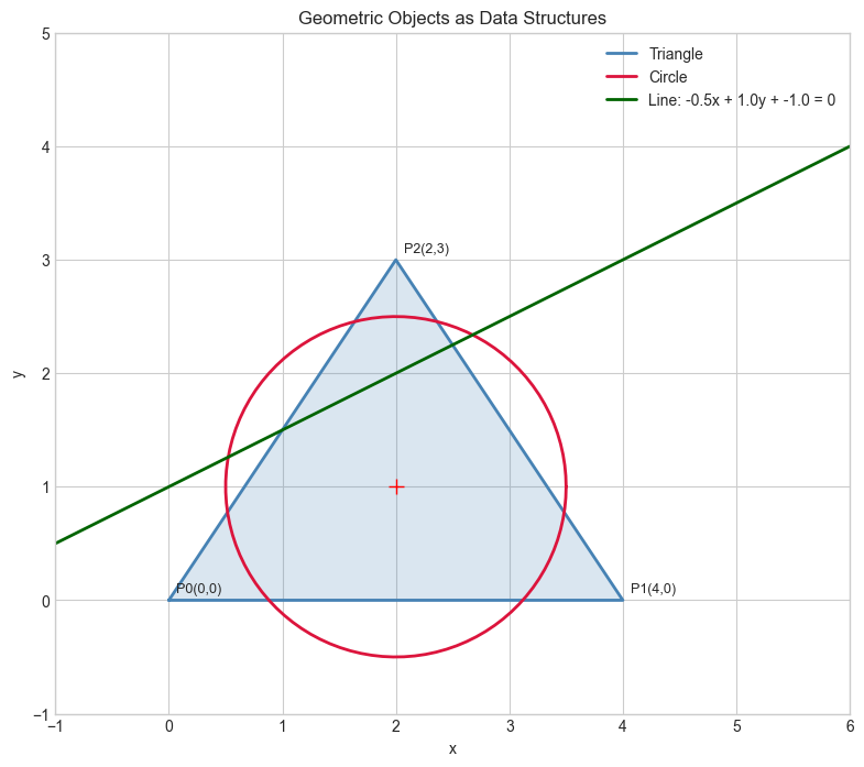
Geometry → ML Connection
Why does geometry appear in ML?
Every data point in a dataset is a point in high-dimensional space.
A 28×28 MNIST image is a point in ℝ^784
Distance between two images = how different they are
The decision boundary of a classifier = a geometric surface (hyperplane, curve, etc.)
This Part builds the 2D intuition. Part V (Vectors) and Part VI (Linear Algebra) generalize to arbitrary dimensions.
Forward connections:
ch094 (Distance) → generalized to norms in ch128 (Vector Length)
ch108–114 (Transformations) → matrix operations in ch164–168
ch103 (Unit Circle) → dot product angles in ch131 (Dot Product)
Summary
Geometric objects are data structures: points as arrays, shapes as collections of points
Geometric operations are functions that transform these data structures
All transformations in 2D are matrix multiplications (proven in ch114)
2D geometry is the foundation for understanding ML’s geometric structure
Next: ch092 — Points and Coordinate Systems