Prerequisites: ch092 (Points and Coordinate Systems)
Outcomes: Operate fluently with 2D and 3D Cartesian coordinates; Understand the four quadrants and sign conventions; Extend to 3D and N-dimensional space
The Cartesian Grid
René Descartes unified algebra and geometry with a single insight: every point corresponds to a unique pair of numbers.
The 2D Cartesian system:
x-axis: horizontal, positive to the right
y-axis: vertical, positive upward
Origin: (0, 0) — intersection of axes
Four quadrants: I (++), II (-+), III (--), IV (+-)
The 3D Cartesian system adds a z-axis (positive toward viewer in right-hand convention).
This correspondence — point ↔ numbers — is what makes computational geometry possible. Without it, we couldn’t represent or compute with shapes.
Quadrants and Practical Ranges
# --- Cartesian coordinate system visualization ---
import numpy as np
import matplotlib.pyplot as plt
plt.style.use('seaborn-v0_8-whitegrid')

fig, axes = plt.subplots(1, 2, figsize=(13, 5))

# 2D quadrant plot
ax = axes[0]
ax.axhline(0, color='black', linewidth=1.5); ax.axvline(0, color='black', linewidth=1.5)
ax.set_xlim(-4, 4); ax.set_ylim(-4, 4)
for text, pos, color in [('Quadrant I(x>0, y>0)',(2,2),'steelblue'),
                          ('Quadrant II(x<0, y>0)',(-2,2),'crimson'),
                          ('Quadrant III(x<0, y<0)',(-2,-2),'darkgreen'),
                          ('Quadrant IV(x>0, y<0)',(2,-2),'darkorange')]:
    ax.text(*pos, text, ha='center', va='center', fontsize=9,
            bbox=dict(boxstyle='round', alpha=0.2, facecolor=color))
# Sample points
for (x,y,label) in [(3,1,'P=(3,1)'),(-2,2.5,'Q=(-2,2.5)'),(-1.5,-2,'R=(-1.5,-2)'),(2.5,-1.5,'S=(2.5,-1.5)')]:
    ax.plot(x,y,'ko',markersize=6)
    ax.annotate(label,(x,y),xytext=(5,5),textcoords='offset points',fontsize=8)
ax.set_xlabel('x'); ax.set_ylabel('y'); ax.set_title('The Four Quadrants')

# 3D coordinate system
ax = axes[1]
ax.set_xlim(-3,4); ax.set_ylim(-3,4)
# Draw axes as arrows (simulated 3D in 2D)
ax.annotate('', xy=(3,0), xytext=(0,0), arrowprops=dict(arrowstyle='->', color='steelblue', lw=2))
ax.annotate('', xy=(0,3), xytext=(0,0), arrowprops=dict(arrowstyle='->', color='crimson', lw=2))
ax.annotate('', xy=(-2,-2), xytext=(0,0), arrowprops=dict(arrowstyle='->', color='darkgreen', lw=2))
ax.text(3.1,0,'x',fontsize=12,color='steelblue',fontweight='bold')
ax.text(0,3.2,'y',fontsize=12,color='crimson',fontweight='bold')
ax.text(-2.3,-2.3,'z',fontsize=12,color='darkgreen',fontweight='bold')
ax.text(0,0,'O',fontsize=11,fontweight='bold')
# A 3D point projected
ax.plot([2],[1],'ko',markersize=8); ax.text(2.1,1.1,'P=(2,1,1.5)',fontsize=9)
ax.plot([0,2],[0,0],'steelblue',lw=1,linestyle='--')
ax.plot([0,0],[0,1],'crimson',lw=1,linestyle='--')
ax.set_title('3D Cartesian System (right-hand)(z comes out toward viewer)')
ax.axis('off')

plt.suptitle('Cartesian Coordinate Systems', fontsize=12, fontweight='bold')
plt.tight_layout(); plt.show()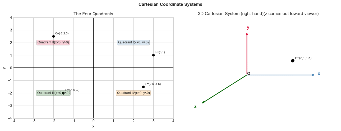
From 2D to N-D
Cartesian coordinates extend naturally to any number of dimensions:
3D: P = (x, y, z) — physical space
4D: P = (x, y, z, t) — spacetime (or 3D + time)
N-D: P = (x₁, x₂, ..., xₙ) — data space in ML
In machine learning, a data point with N features is a point in ℝᴺ. The Cartesian framework extends: distances, angles, and transformations all generalize. The intuition you build in 2D carries directly.
(Generalized distances in ch128; N-dimensional vectors in ch121–127.)
Summary
Cartesian coordinates: P = (x, y), four quadrants, origin at (0,0)
3D extends with z-axis (right-hand convention: x right, y up, z toward you)
N-dimensional generalization: each feature in ML is a coordinate axis
The Cartesian framework is the universal language of computational geometry
Forward: ch094 computes distances between Cartesian points. The distance formula comes directly from the Pythagorean theorem.