Chapter 126 — Scalar Multiplication - Mathematics for Programmers

Prerequisites: Vector Addition (ch125), What is a Vector? (ch121) You will learn:
What scalar multiplication does geometrically and algebraically
How negative scalars reverse direction
The distributive laws that connect scalar multiplication and addition
Why scalar multiplication is one of the two axioms underlying all of vector algebra

Environment: Python 3.x, numpy, matplotlib

1. Concept¶

Scalar multiplication scales a vector by a real number. Multiply each component by the scalar.

c \mathbf{v} = \begin{pmatrix} c v_1 \\ c v_2 \\ \vdots \\ c v_n \end{pmatrix}

(1)

Geometrically:

If $c > 1$ : the vector grows longer, same direction.
If $0 < c < 1$ : the vector shrinks, same direction.
If $c = -1$ : the vector flips to the opposite direction, same length.
If $c < 0$ : the vector flips and scales.
If $c = 0$ : the vector collapses to the zero vector.

Common misconception: Scalar multiplication does not change the direction of a vector when $c > 0$ . Direction only flips when $c < 0$ . Scaling and direction change are independent effects.

2. Intuition & Mental Models¶

Geometric model: Think of a vector as a rubber band stretched in a specific direction. Multiplying by 2 doubles the stretch. Multiplying by 0.5 halves it. Multiplying by −1 flips the band to point the opposite way.

Physical model: A force of 10N north is the same direction as 3N north — they are scalar multiples of the same unit vector (one pointing north). Scaling the force means scaling the magnitude.

Computational model: Think of a vector as a template arrow. Any scalar multiple is a stretched/flipped/shrunk version of the same template, still lying on the same line through the origin.

Recall from ch125 (Vector Addition) that $-\mathbf{v}$ is the additive inverse. That is exactly $(-1) \cdot \mathbf{v}$ — scalar multiplication with $c = -1$ .

3. Visualization¶

# --- Visualization: Effect of different scalars on a vector ---
import numpy as np
import matplotlib.pyplot as plt
plt.style.use('seaborn-v0_8-whitegrid')

v = np.array([2.0, 1.0])
scalars = [2.0, 1.0, 0.5, 0.0, -0.5, -1.0, -2.0]

colors = plt.cm.coolwarm(np.linspace(0, 1, len(scalars)))

fig, ax = plt.subplots(figsize=(8, 6))

for c, color in zip(scalars, colors):
    scaled = c * v
    ax.annotate('', xy=scaled, xytext=[0, 0],
                arrowprops=dict(arrowstyle='->', color=color, lw=2.0))
    if c != 0:
        ax.text(scaled[0]*1.05, scaled[1]*1.05, f'c={c}', fontsize=9, color=color)

ax.plot(0, 0, 'ko', markersize=5)
ax.set_xlim(-5, 5); ax.set_ylim(-3, 3)
ax.axhline(0, color='black', lw=0.7); ax.axvline(0, color='black', lw=0.7)
ax.set_aspect('equal')
ax.set_title('Scalar multiples of v = [2, 1]')
ax.set_xlabel('x'); ax.set_ylabel('y')
plt.tight_layout()
plt.show()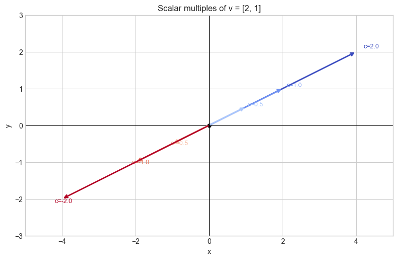

4. Mathematical Formulation¶

Definition. For $c \in \mathbb{R}$ and $\mathbf{v} \in \mathbb{R}^n$ :

(c\mathbf{v})_i = c \cdot v_i \qquad \text{for all } i

(2)

Properties (Distributive laws):

$c(\mathbf{u} + \mathbf{v}) = c\mathbf{u} + c\mathbf{v}$ — scalar distributes over vector addition
$(a + b)\mathbf{v} = a\mathbf{v} + b\mathbf{v}$ — vector distributes over scalar addition
$a(b\mathbf{v}) = (ab)\mathbf{v}$ — scalar multiplication is associative with scalars
$1 \cdot \mathbf{v} = \mathbf{v}$ — multiplicative identity

Together with vector addition properties (ch125), these eight axioms define a vector space (formalized in ch137).

# --- Mathematical Formulation: verify distributive laws ---
import numpy as np

u = np.array([1.0, 3.0, -2.0])
v = np.array([2.0, -1.0, 4.0])
a, b, c = 2.5, -1.0, 3.0

print("Distributive (scalar over vector sum):")
lhs = c * (u + v)
rhs = c * u + c * v
print(f"  c*(u+v) = {lhs}")
print(f"  c*u+c*v = {rhs}")
print(f"  Equal?   {np.allclose(lhs, rhs)}")

print("\nDistributive (vector over scalar sum):")
lhs = (a + b) * v
rhs = a * v + b * v
print(f"  (a+b)*v = {lhs}")
print(f"  a*v+b*v = {rhs}")
print(f"  Equal?   {np.allclose(lhs, rhs)}")

print("\nAssociativity with scalars:")
print(f"  a*(b*v) = {a*(b*v)}")
print(f"  (a*b)*v = {(a*b)*v}")
print(f"  Equal?   {np.allclose(a*(b*v), (a*b)*v)}")

Distributive (scalar over vector sum):
  c*(u+v) = [9. 6. 6.]
  c*u+c*v = [9. 6. 6.]
  Equal?   True

Distributive (vector over scalar sum):
  (a+b)*v = [ 3.  -1.5  6. ]
  a*v+b*v = [ 3.  -1.5  6. ]
  Equal?   True

Associativity with scalars:
  a*(b*v) = [ -5.    2.5 -10. ]
  (a*b)*v = [ -5.    2.5 -10. ]
  Equal?   True

5. Python Implementation¶

# --- Implementation: scalar_multiply and unit vector ---
import numpy as np

def scalar_multiply(c, v):
    """
    Multiply vector v by scalar c.

    Args:
        c: float — the scalar
        v: ndarray shape (n,)

    Returns:
        ndarray shape (n,)
    """
    v = np.asarray(v, dtype=float)
    return np.array([c * vi for vi in v])


def normalize(v):
    """
    Return the unit vector in the direction of v (scale to magnitude 1).
    This is scalar multiplication by 1/||v||.

    Args:
        v: ndarray shape (n,), must be non-zero

    Returns:
        ndarray shape (n,)

    Raises:
        ValueError: if v is the zero vector
    """
    mag = np.linalg.norm(v)
    if mag < 1e-12:
        raise ValueError("Cannot normalize the zero vector.")
    return v / mag  # equivalent to scalar_multiply(1/mag, v)


v = np.array([3.0, 4.0])
scaled = scalar_multiply(2.5, v)
unit   = normalize(v)

print("v =", v)
print("2.5 * v =", scaled)
print("unit(v) =", unit, "  magnitude:", np.linalg.norm(unit))

# Verify: scalar_multiply(||v||, unit(v)) should recover v
mag = np.linalg.norm(v)
recovered = scalar_multiply(mag, unit)
print("mag * unit(v) =", recovered, " match:", np.allclose(recovered, v))

v = [3. 4.]
2.5 * v = [ 7.5 10. ]
unit(v) = [0.6 0.8]   magnitude: 1.0
mag * unit(v) = [3. 4.]  match: True

6. Experiments¶

# --- Experiment 1: Direction is preserved under positive scaling ---
# Hypothesis: the angle between v and c*v is 0 for c > 0, and 180° for c < 0.
# Try changing: the scalar c.
import numpy as np

v = np.array([3.0, 2.0])
C_VALUES = [3.0, 1.0, 0.1, -0.1, -1.0, -3.0]  # <-- modify

for c in C_VALUES:
    scaled = c * v
    # dot product / product of magnitudes = cos(angle)
    cos_angle = np.dot(v, scaled) / (np.linalg.norm(v) * np.linalg.norm(scaled))
    angle_deg = np.degrees(np.arccos(np.clip(cos_angle, -1, 1)))
    print(f"c={c:5.1f}  scaled={scaled}  angle={angle_deg:.1f}°")

c=  3.0  scaled=[9. 6.]  angle=0.0°
c=  1.0  scaled=[3. 2.]  angle=0.0°
c=  0.1  scaled=[0.3 0.2]  angle=0.0°
c= -0.1  scaled=[-0.3 -0.2]  angle=180.0°
c= -1.0  scaled=[-3. -2.]  angle=180.0°
c= -3.0  scaled=[-9. -6.]  angle=180.0°

# --- Experiment 2: Unit vectors ---
# Hypothesis: any non-zero vector divided by its norm produces a vector of length 1.
# Try changing: the vector v.
import numpy as np

v = np.array([7.0, -3.0, 2.0])  # <-- modify: try different magnitudes

unit_v = v / np.linalg.norm(v)
print("v:         ", v)
print("||v||:     ", np.linalg.norm(v))
print("unit(v):   ", unit_v)
print("||unit(v)||:", np.linalg.norm(unit_v))

v:          [ 7. -3.  2.]
||v||:      7.874007874011811
unit(v):    [ 0.88900089 -0.38100038  0.25400025]
||unit(v)||: 0.9999999999999999

7. Exercises¶

Easy 1. Compute $3 \cdot (2, -1, 4)$ and $(-0.5) \cdot (6, 0, -2)$ by hand, then verify with NumPy. (Expected: (6, -3, 12) and (-3, 0, 1))

Easy 2. Normalize the vector v = (1, 1). What is the result? What angle does it make with the x-axis? (Expected: (0.707, 0.707), 45°)

Medium 1. Write a function scale_to_length(v, target_length) that scales v to have magnitude target_length. Verify on v = (3, 4) with target 10.

Medium 2. Generate 100 random 3D vectors. Normalize each one. Verify that all normalized vectors lie on the unit sphere by checking their norms.

Hard. Prove algebraically that scalar multiplication distributes over vector addition: $c(\mathbf{u} + \mathbf{v}) = c\mathbf{u} + c\mathbf{v}$ . What property of real numbers does this rely on? (Challenge: connect to the distributive law for real numbers)

8. Mini Project¶

# --- Mini Project: Vector Animation Path ---
# Problem: Animate an object moving along a direction vector at variable speeds.
#          Scalar multiplication controls speed (magnitude) while direction stays fixed.
# Task: generate position frames using direction vector + scalar speed control.

import numpy as np
import matplotlib.pyplot as plt
plt.style.use('seaborn-v0_8-whitegrid')

# Constant direction (normalized)
direction = np.array([1.0, 0.5])
direction = direction / np.linalg.norm(direction)  # unit vector

# Speed at each time step (variable — scalar multiplier)
T = 50
t = np.linspace(0, 2*np.pi, T)
speeds = 1.0 + 0.8 * np.sin(t)  # oscillating speed: 0.2 to 1.8

# TODO: compute positions
# positions[k] = positions[k-1] + speeds[k] * direction
# Start at origin.

# Starter:
positions = np.zeros((T, 2))
for k in range(1, T):
    positions[k] = positions[k-1] + speeds[k] * direction  # <-- fill this

fig, axes = plt.subplots(1, 2, figsize=(12, 4))

axes[0].plot(positions[:, 0], positions[:, 1], 'o-', markersize=3, color='steelblue')
axes[0].plot(*positions[0], 'go', markersize=8); axes[0].plot(*positions[-1], 'r*', markersize=10)
axes[0].set_title('Path (direction fixed, speed varies)')
axes[0].set_xlabel('x'); axes[0].set_ylabel('y')
axes[0].set_aspect('equal')

axes[1].plot(t, speeds, color='coral')
axes[1].set_title('Speed vs Time (scalar multiplier)')
axes[1].set_xlabel('Time'); axes[1].set_ylabel('Speed')

plt.tight_layout()
plt.show()

9. Summary & Connections¶

Scalar multiplication scales a vector’s magnitude; it preserves direction for $c > 0$ , reverses it for $c < 0$ .
The unit vector $\hat{\mathbf{v}} = \mathbf{v} / \|\mathbf{v}\|$ encodes direction only (magnitude = 1).
Distributive laws: $c(\mathbf{u}+\mathbf{v}) = c\mathbf{u}+c\mathbf{v}$ and $(a+b)\mathbf{v} = a\mathbf{v}+b\mathbf{v}$ .

Backward connection: The additive inverse $-\mathbf{v}$ from ch125 is scalar multiplication by -1.

Forward connections:

This will reappear in ch127 — Linear Combination, where vectors are scaled and summed simultaneously.
This will reappear in ch128 — Vector Length, where the norm of $c\mathbf{v}$ equals $|c|\|\mathbf{v}\|$ — scalar multiplication scales the norm by $|c|$ .
This will reappear in ch212 — Gradient Descent (Part VII), where parameters are updated by $\theta \leftarrow \theta - \alpha \nabla L$ — scalar multiplication of the gradient.