Prerequisites: Vector Addition (ch125), Scalar Multiplication (ch126) You will learn:
The definition of a linear combination of vectors
Why linear combinations are the fundamental operation of linear algebra
How to compute them efficiently with NumPy
Applications: interpolation, weighted averages, and color mixing
Environment: Python 3.x, numpy, matplotlib
1. Concept
A linear combination of vectors is any vector of the form:
where are scalars called coefficients or weights.
This is simply scaling each vector and adding the results. But the concept is vastly more important than it sounds. Almost every operation in linear algebra — matrix-vector multiplication, projections, regression, neural network layers — is ultimately a linear combination.
Common misconception: A linear combination does not require the vectors to be linearly independent, nor the coefficients to sum to 1. Both are special cases.
2. Intuition & Mental Models
Color model: RGB colors are linear combinations of the basis colors red, green, blue. The color (255, 128, 0) is .
Mixing model: Imagine mixing paints. Each paint is a vector (its color). A linear combination is a recipe: “3 parts this, 1 part that.” The result is a new paint.
Coordinate model: Every vector in ℝⁿ is a linear combination of the standard basis vectors: . You use this every time you write coordinates.
Recall from ch126 (Scalar Multiplication): the scaling step. Recall from ch125 (Vector Addition): the summing step. A linear combination is both, combined.
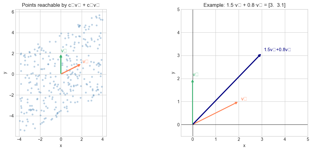
3. Visualization
# --- Visualization: Linear combinations of two vectors ---
# Show what region is reachable by varying c1 and c2
import numpy as np
import matplotlib.pyplot as plt
plt.style.use('seaborn-v0_8-whitegrid')

v1 = np.array([2.0, 1.0])
v2 = np.array([0.0, 2.0])

# Sample many coefficient pairs and plot the resulting combinations
np.random.seed(0)
N = 300
c1_vals = np.random.uniform(-2, 2, N)
c2_vals = np.random.uniform(-2, 2, N)

# Each row: c1*v1 + c2*v2
points = np.outer(c1_vals, v1) + np.outer(c2_vals, v2)

fig, axes = plt.subplots(1, 2, figsize=(13, 5))

# ---- Left: scatter of reachable points ----
ax = axes[0]
ax.scatter(points[:, 0], points[:, 1], alpha=0.3, s=10, color='steelblue')
ax.annotate('', xy=v1, xytext=[0, 0],
            arrowprops=dict(arrowstyle='->', color='coral', lw=2.5))
ax.annotate('', xy=v2, xytext=[0, 0],
            arrowprops=dict(arrowstyle='->', color='mediumseagreen', lw=2.5))
ax.text(*v1*1.05, 'v₁', color='coral', fontsize=12)
ax.text(*v2*1.05, 'v₂', color='mediumseagreen', fontsize=12)
ax.set_title('Points reachable by c₁v₁ + c₂v₂')
ax.set_xlabel('x'); ax.set_ylabel('y')
ax.set_aspect('equal')

# ---- Right: specific example c1=1.5, c2=0.8 ----
ax = axes[1]
C1, C2 = 1.5, 0.8
result = C1 * v1 + C2 * v2

for vec, label, color in [(v1, 'v₁', 'coral'), (v2, 'v₂', 'mediumseagreen')]:
    ax.annotate('', xy=vec, xytext=[0, 0],
                arrowprops=dict(arrowstyle='->', color=color, lw=2))
    ax.text(*vec*1.05, label, color=color, fontsize=12)

ax.annotate('', xy=result, xytext=[0, 0],
            arrowprops=dict(arrowstyle='->', color='navy', lw=2.5))
ax.text(*result*1.03, f'{C1}v₁+{C2}v₂', color='navy', fontsize=11)

ax.set_xlim(-0.5, 5); ax.set_ylim(-0.5, 5)
ax.axhline(0, color='black', lw=0.7); ax.axvline(0, color='black', lw=0.7)
ax.set_aspect('equal')
ax.set_title(f'Example: {C1}·v₁ + {C2}·v₂ = {result}')
ax.set_xlabel('x'); ax.set_ylabel('y')

plt.tight_layout()
plt.show()
C:\Users\user\AppData\Local\Temp\ipykernel_1940\3657564691.py:54: UserWarning: Glyph 8321 (\N{SUBSCRIPT ONE}) missing from font(s) Arial.
plt.tight_layout()
C:\Users\user\AppData\Local\Temp\ipykernel_1940\3657564691.py:54: UserWarning: Glyph 8322 (\N{SUBSCRIPT TWO}) missing from font(s) Arial.
plt.tight_layout()
c:\Users\user\OneDrive\Documents\book\.venv\Lib\site-packages\IPython\core\pylabtools.py:170: UserWarning: Glyph 8321 (\N{SUBSCRIPT ONE}) missing from font(s) Arial.
fig.canvas.print_figure(bytes_io, **kw)
c:\Users\user\OneDrive\Documents\book\.venv\Lib\site-packages\IPython\core\pylabtools.py:170: UserWarning: Glyph 8322 (\N{SUBSCRIPT TWO}) missing from font(s) Arial.
fig.canvas.print_figure(bytes_io, **kw)
4. Mathematical Formulation
Definition. Given vectors and scalars , their linear combination is:
Special cases:
Affine combination: — the result lies on the affine hull (e.g., the line or plane through the vectors)
Convex combination: and — the result lies between the vectors (interpolation)
Span: the set of all possible linear combinations of is their span (ch140)
As matrix-vector product: if the vectors are columns of a matrix , then computes the linear combination — this is the fundamental insight connecting vectors to matrices (ch151–153, Part VI).
# --- Mathematical Formulation: linear_combination ---
import numpy as np

def linear_combination(vectors, coefficients):
    """
    Compute the linear combination sum(c_j * v_j).

    Args:
        vectors: list of ndarrays, each shape (n,)
        coefficients: list of floats, same length

    Returns:
        ndarray shape (n,)
    """
    vectors = [np.asarray(v, float) for v in vectors]
    n = vectors[0].shape[0]
    result = np.zeros(n)
    for c, v in zip(coefficients, vectors):
        result = result + c * v
    return result


v1 = np.array([1.0, 0.0, 0.0])  # e1
v2 = np.array([0.0, 1.0, 0.0])  # e2
v3 = np.array([0.0, 0.0, 1.0])  # e3

# Any vector is a linear combination of basis vectors
target = np.array([3.0, -2.0, 5.0])
result = linear_combination([v1, v2, v3], [3, -2, 5])
print("target:", target)
print("result:", result)
print("match: ", np.allclose(target, result))

# Convex combination (coefficients sum to 1): midpoint
a = np.array([0.0, 0.0])
b = np.array([4.0, 2.0])
midpoint = linear_combination([a, b], [0.5, 0.5])
print("\nMidpoint of a and b:", midpoint)
target: [ 3. -2. 5.]
result: [ 3. -2. 5.]
match: True
Midpoint of a and b: [2. 1.]
5. Python Implementation
# --- Implementation: Efficient vectorized linear combination ---
import numpy as np

def linear_combination_fast(V, c):
    """
    Compute linear combination using matrix-vector product.
    Equivalent to sum(c[j] * V[j] for all j).

    Args:
        V: ndarray shape (k, n) — k vectors of dimension n, one per row
        c: ndarray shape (k,)   — k coefficients

    Returns:
        ndarray shape (n,)
    """
    V = np.asarray(V, dtype=float)
    c = np.asarray(c, dtype=float)
    # V.T @ c is equivalent to sum(c[j] * V[j])
    return V.T @ c


def interpolate(u, v, t):
    """
    Linear interpolation between u (t=0) and v (t=1).
    This is a convex combination: (1-t)*u + t*v.

    Args:
        u, v: ndarray shape (n,)
        t: float in [0, 1]

    Returns:
        ndarray shape (n,)
    """
    return (1 - t) * np.asarray(u, float) + t * np.asarray(v, float)


# Test
V = np.array([[1.0, 0.0], [0.0, 1.0], [1.0, 1.0]])
c = np.array([2.0, -1.0, 0.5])
print("Linear combination:", linear_combination_fast(V, c))

u = np.array([0.0, 0.0])
v = np.array([10.0, 5.0])
for t in [0.0, 0.25, 0.5, 0.75, 1.0]:
    pt = interpolate(u, v, t)
    print(f"t={t:.2f}  →  {pt}")
Linear combination: [ 2.5 -0.5]
t=0.00 → [0. 0.]
t=0.25 → [2.5 1.25]
t=0.50 → [5. 2.5]
t=0.75 → [7.5 3.75]
t=1.00 → [10. 5.]
6. Experiments
# --- Experiment 1: Color mixing as linear combination ---
# Hypothesis: RGB colors are linear combinations of basis colors.
# Try changing: the coefficients to mix different colors.
import numpy as np
import matplotlib.pyplot as plt
plt.style.use('seaborn-v0_8-whitegrid')

red   = np.array([1.0, 0.0, 0.0])
green = np.array([0.0, 1.0, 0.0])
blue  = np.array([0.0, 0.0, 1.0])

# Coefficients (must be in [0,1] for valid RGB)
C_RED   = 0.8  # <-- modify
C_GREEN = 0.3  # <-- modify
C_BLUE  = 0.5  # <-- modify

mixed = np.clip(C_RED * red + C_GREEN * green + C_BLUE * blue, 0, 1)

fig, axes = plt.subplots(1, 4, figsize=(10, 2))
for ax, color, title in zip(axes,
    [red, green, blue, mixed],
    ['Red', 'Green', 'Blue', f'Mix ({C_RED:.1f}R+{C_GREEN:.1f}G+{C_BLUE:.1f}B)']):
    ax.set_facecolor(color)
    ax.set_title(title, fontsize=9)
    ax.set_xticks([]); ax.set_yticks([])

plt.suptitle('Colors as Linear Combinations of RGB Basis Vectors', y=1.05)
plt.tight_layout()
plt.show()
print("Mixed color (RGB):", mixed)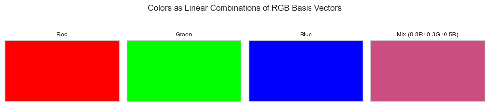
Mixed color (RGB): [0.8 0.3 0.5]
# --- Experiment 2: Interpolation path ---
# Hypothesis: varying t from 0 to 1 traces a straight line between two points.
# Try changing: T_VALUES to non-uniform spacings.
import numpy as np
import matplotlib.pyplot as plt
plt.style.use('seaborn-v0_8-whitegrid')

start = np.array([0.0, 0.0])
end   = np.array([5.0, 3.0])

T_VALUES = np.linspace(0, 1, 20)  # <-- modify: try np.logspace, custom values

pts = np.array([(1-t)*start + t*end for t in T_VALUES])

plt.figure(figsize=(7, 4))
plt.scatter(pts[:, 0], pts[:, 1], c=T_VALUES, cmap='viridis', s=50)
plt.colorbar(label='t value')
plt.plot(*start, 'go', markersize=8); plt.plot(*end, 'r*', markersize=10)
plt.title('Interpolation: (1-t)·start + t·end')
plt.xlabel('x'); plt.ylabel('y')
plt.tight_layout(); plt.show()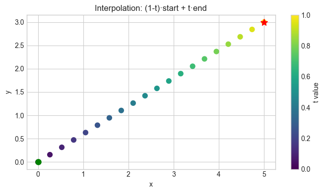
7. Exercises
Easy 1. Compute for u = (1,0,2), v = (3,1,-1), w = (0,4,0). (Expected: (-7, 1, 7))
Easy 2. Express the vector (5, 3) as a linear combination of (1, 0) and (0, 1). Then express it as a linear combination of (1, 1) and (1, -1). Hint for the second: solve the 2×2 system.
Medium 1. Implement weighted_average(vectors, weights) where weights are non-negative and sum to 1. Apply it to compute the centroid of 5 random 2D points.
Medium 2. Generate 50 interpolation frames between two 3D points p = (0,0,0) and q = (1,2,3). Plot the trajectory in 3D using ax = fig.add_subplot(projection='3d').
Hard. Show that every vector in ℝ³ can be written as a linear combination of v₁ = (1,1,0), v₂ = (1,0,1), v₃ = (0,1,1). Find the coefficients for w = (3,5,1). (Challenge: solve the 3×3 linear system — relates to ch160, Gaussian Elimination)
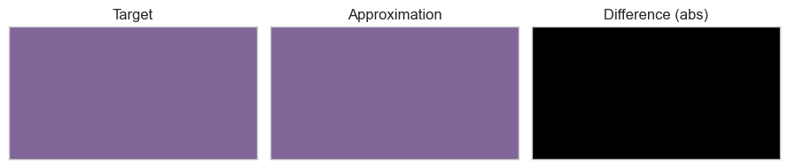
8. Mini Project
# --- Mini Project: Palette Mixer ---
# Problem: Given a target RGB color, find the closest mixture of 3 palette colors.
# This is a constrained linear combination problem.
# Task: implement find_mixture() using least squares, visualize result.

import numpy as np
import matplotlib.pyplot as plt
plt.style.use('seaborn-v0_8-whitegrid')

# Palette: 3 paint colors (normalized RGB)
palette = np.array([
    [0.9, 0.1, 0.1],  # red-ish
    [0.1, 0.7, 0.2],  # green-ish
    [0.1, 0.2, 0.9],  # blue-ish
])

target = np.array([0.5, 0.4, 0.6])  # the color we want to approximate

def find_mixture(palette, target):
    """
    Find coefficients c such that palette.T @ c ≈ target.
    Use np.linalg.lstsq to find least-squares solution.

    Args:
        palette: ndarray shape (k, 3) — k paint colors
        target:  ndarray shape (3,)   — target RGB

    Returns:
        c: ndarray shape (k,) — mixture coefficients
        approximation: ndarray shape (3,) — achieved color
    """
    # palette.T @ c = target
    c, _, _, _ = np.linalg.lstsq(palette.T, target, rcond=None)
    approx = palette.T @ c
    return c, np.clip(approx, 0, 1)


coefficients, approximation = find_mixture(palette, target)
print("Coefficients:", coefficients)
print("Approximation:", approximation)
print("Target:       ", target)
print("Error:        ", np.linalg.norm(target - approximation))

fig, axes = plt.subplots(1, 3, figsize=(9, 2))
for ax, color, title in zip(axes,
    [target, approximation, np.abs(target - approximation)],
    ['Target', 'Approximation', 'Difference (abs)']):
    ax.set_facecolor(color)
    ax.set_title(title)
    ax.set_xticks([]); ax.set_yticks([])
plt.tight_layout(); plt.show()
Coefficients: [0.4566474 0.35260116 0.53757225]
Approximation: [0.5 0.4 0.6]
Target: [0.5 0.4 0.6]
Error: 3.3766115072321297e-16
9. Summary & Connections
A linear combination is a sum of scaled vectors: .
Special cases: convex combination (, ) stays between the vectors.
The set of all linear combinations of a set of vectors is their span (formalized in ch140).
The matrix-vector product computes a linear combination of the columns of .
Backward connection: This combines ch125 (addition) and ch126 (scaling) into the central operation of all linear algebra.
Forward connections:
This will reappear in ch140 — Span, where we ask: what is the set of all possible linear combinations of a given set of vectors?
This will reappear in ch153 — Matrix Multiplication (Part VI), where every column of is a linear combination of columns of .
This will reappear in ch177 — Linear Layers in Deep Learning, where a neural network layer computes a learned linear combination of inputs.