Prerequisites: ch131 (dot product intuition), ch128 (norms), ch112 (trigonometry/unit circle)
You will learn:
Why
How to derive this from the law of cosines
How the sign of the dot product tells you which half-space a vector lives in
How to extract angles from vectors using the dot product
Environment: Python 3.x, numpy, matplotlib
1. Concept
In ch131, we defined the dot product algebraically: . We observed that it behaves like an alignment score. This chapter proves why.
The geometric formula is:
where is the angle between the two vectors.
This connects three things: the sizes of the two vectors, the angle between them, and the scalar output. None of these alone determines the dot product — all three together do.
Common misconceptions:
The formula gives (0 to 180 degrees), not the full circle. Vectors do not have a signed direction of rotation between them.
When or is the zero vector, the angle is undefined. The dot product is zero, but not because of orthogonality.
2. Intuition & Mental Models
Physical: A solar panel generates maximum power when it faces the sun directly (, ). Tilted at 90 degrees it generates nothing (). Facing away, it generates negative (relative) contribution (). The dot product is the formula for this.
Geometric: Think of the dot product as: how much of would I measure if I used 's direction as my ruler? The answer is — the signed projection length — scaled by . (Projection formalized in ch134.)
Computational: The formula is how machines measure similarity. Divide out the magnitudes and you get a scale-free angle measure — cosine similarity. This is used in every search engine and recommendation system.
Recall from ch112 (Sine and Cosine) that oscillates between -1 and 1, peaking at and reaching -1 at . The dot product inherits this shape exactly.
3. Visualization
# --- Visualization: Angle between vectors and dot product formula ---

import numpy as np
import matplotlib.pyplot as plt
import matplotlib.patches as mpatches

plt.style.use('seaborn-v0_8-whitegrid')

def draw_angle_arc(ax, v1, v2, radius=0.3, color='purple'):
    """Draw a small arc showing the angle between two vectors from origin."""
    angle1 = np.degrees(np.arctan2(v1[1], v1[0]))
    angle2 = np.degrees(np.arctan2(v2[1], v2[0]))
    if angle1 > angle2:
        angle1, angle2 = angle2, angle1
    arc = mpatches.Arc([0, 0], 2*radius, 2*radius,
                        angle=0, theta1=angle1, theta2=angle2,
                        color=color, linewidth=1.5)
    ax.add_patch(arc)

fig, axes = plt.subplots(1, 3, figsize=(14, 5))

test_cases = [
    (np.array([2.0, 0.5]), np.array([1.5, 1.5])),
    (np.array([2.0, 0.0]), np.array([0.0, 2.0])),
    (np.array([2.0, 0.5]), np.array([-1.5, -0.5])),
]

ORIGIN = np.array([0, 0])

for ax, (a, b) in zip(axes, test_cases):
    dot = np.dot(a, b)
    cos_theta = dot / (np.linalg.norm(a) * np.linalg.norm(b))
    theta_deg = np.degrees(np.arccos(np.clip(cos_theta, -1, 1)))

    ax.quiver(*ORIGIN, *a, angles='xy', scale_units='xy', scale=1,
               color='steelblue', width=0.012, label='a')
    ax.quiver(*ORIGIN, *b, angles='xy', scale_units='xy', scale=1,
               color='tomato', width=0.012, label='b')
    draw_angle_arc(ax, a, b)
    ax.set_xlim(-2.5, 2.5)
    ax.set_ylim(-2.5, 2.5)
    ax.set_aspect('equal')
    ax.axhline(0, color='gray', linewidth=0.4)
    ax.axvline(0, color='gray', linewidth=0.4)
    ax.set_title(
        f'θ = {theta_deg:.1f}°\ncos θ = {cos_theta:.3f}\na·b = {dot:.2f}',
        fontsize=10)
    ax.legend(fontsize=8)
    ax.set_xlabel('x'); ax.set_ylabel('y')

plt.suptitle('Geometric Formula: a·b = ||a|| ||b|| cos θ', fontsize=13, fontweight='bold')
plt.tight_layout()
plt.show()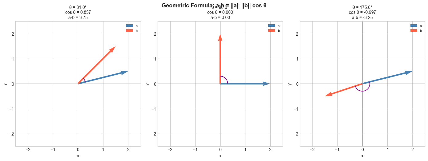
# --- Visualization: Cosine similarity heatmap ---
# Create several named vectors, compute all pairwise cosine similarities.

labels = ['East', 'NE', 'North', 'NW', 'West', 'SW']
angles_deg_map = [0, 45, 90, 135, 180, 225]
vectors = np.array([[np.cos(np.radians(a)), np.sin(np.radians(a))]
                     for a in angles_deg_map])

# Compute pairwise cosine similarities
n = len(vectors)
sim_matrix = np.zeros((n, n))
for i in range(n):
    for j in range(n):
        dot = np.dot(vectors[i], vectors[j])
        norms = np.linalg.norm(vectors[i]) * np.linalg.norm(vectors[j])
        sim_matrix[i, j] = dot / norms

fig, ax = plt.subplots(figsize=(7, 6))
im = ax.imshow(sim_matrix, cmap='RdBu', vmin=-1, vmax=1)
ax.set_xticks(range(n)); ax.set_xticklabels(labels)
ax.set_yticks(range(n)); ax.set_yticklabels(labels)
plt.colorbar(im, ax=ax, label='Cosine similarity')
for i in range(n):
    for j in range(n):
        ax.text(j, i, f'{sim_matrix[i,j]:.2f}', ha='center', va='center', fontsize=9)
ax.set_title('Pairwise Cosine Similarity of Compass Directions')
plt.tight_layout()
plt.show()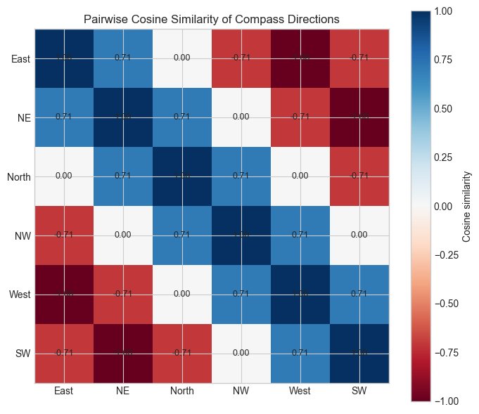
4. Mathematical Formulation
Derivation via the Law of Cosines
Consider vectors and and the vector , forming a triangle.
The law of cosines states:
Expand using dot product properties (from the Hard exercise in ch131):
Setting equal:
Cancel and solve:
Rearranged as the angle formula:
Cosine similarity (scale-free version):
5. Python Implementation
# --- Implementation: angle_between and cosine_similarity ---

def angle_between(a, b, degrees=False):
    """
    Compute the angle between two non-zero vectors.

    Args:
        a, b:    array-like, shape (n,), must be non-zero
        degrees: if True, return angle in degrees; else radians

    Returns:
        float: angle in [0, π] radians (or [0, 180] degrees)
    """
    a, b = np.asarray(a, dtype=float), np.asarray(b, dtype=float)
    cos_theta = np.dot(a, b) / (np.linalg.norm(a) * np.linalg.norm(b))
    # Clip to [-1, 1] to guard against floating point errors like cos=1.0000000002
    cos_theta = np.clip(cos_theta, -1.0, 1.0)
    theta = np.arccos(cos_theta)
    return np.degrees(theta) if degrees else theta


def cosine_similarity(a, b):
    """
    Scale-free similarity measure between two vectors.

    Returns:
        float in [-1, 1]; 1 = identical direction, -1 = opposite
    """
    a, b = np.asarray(a, dtype=float), np.asarray(b, dtype=float)
    return np.dot(a, b) / (np.linalg.norm(a) * np.linalg.norm(b))


# Test cases
print("Angle tests:")
print(f"  [1,0] vs [1,0]:  {angle_between([1,0],[1,0], degrees=True):.1f}°  (expect 0)")
print(f"  [1,0] vs [0,1]:  {angle_between([1,0],[0,1], degrees=True):.1f}°  (expect 90)")
print(f"  [1,0] vs [-1,0]: {angle_between([1,0],[-1,0], degrees=True):.1f}° (expect 180)")
print(f"  [1,1] vs [1,0]:  {angle_between([1,1],[1,0], degrees=True):.1f}°  (expect 45)")

print("\nCosine similarity tests:")
print(f"  [1,2,3] vs [2,4,6]: {cosine_similarity([1,2,3],[2,4,6]):.4f}  (expect 1.0 — same direction)")
print(f"  [1,0]   vs [0,1]:   {cosine_similarity([1,0],[0,1]):.4f}  (expect 0.0 — orthogonal)")
Angle tests:
[1,0] vs [1,0]: 0.0° (expect 0)
[1,0] vs [0,1]: 90.0° (expect 90)
[1,0] vs [-1,0]: 180.0° (expect 180)
[1,1] vs [1,0]: 45.0° (expect 45)
Cosine similarity tests:
[1,2,3] vs [2,4,6]: 1.0000 (expect 1.0 — same direction)
[1,0] vs [0,1]: 0.0000 (expect 0.0 — orthogonal)
# --- Half-space classifier using dot product sign ---
# Given a direction vector w, classify points as positive/negative
# based on which side of the hyperplane through the origin they lie on.
# This is the geometric foundation of the perceptron (ch176).

np.random.seed(7)
N = 200
points = np.random.randn(N, 2)  # random 2D points

w = np.array([1.0, 0.5])  # decision direction vector
w_hat = w / np.linalg.norm(w)  # normalize for display

# Sign of dot product with w determines class
scores = points @ w  # dot product of each point with w
labels = (scores >= 0).astype(int)  # 1 if positive side, 0 if negative

fig, ax = plt.subplots(figsize=(7, 6))
colors = ['tomato' if l == 0 else 'steelblue' for l in labels]
ax.scatter(points[:, 0], points[:, 1], c=colors, alpha=0.6, s=20)

# Draw the decision boundary (perpendicular to w, through origin)
t = np.linspace(-3, 3, 100)
boundary = np.array([-w[1], w[0]])  # perpendicular to w
boundary /= np.linalg.norm(boundary)
ax.plot(t * boundary[0], t * boundary[1], 'k--', linewidth=1.5, label='Decision boundary')

# Draw w
ax.quiver(0, 0, w_hat[0], w_hat[1], angles='xy', scale_units='xy', scale=1,
           color='black', width=0.015, label=f'w = {w}')

from matplotlib.patches import Patch
ax.legend(handles=[
    Patch(color='steelblue', label='w·x ≥ 0 (positive side)'),
    Patch(color='tomato',    label='w·x < 0 (negative side)'),
], loc='upper left')
ax.set_xlim(-3, 3); ax.set_ylim(-3, 3)
ax.set_aspect('equal')
ax.set_title('Half-Space Classification via Dot Product Sign')
ax.set_xlabel('x'); ax.set_ylabel('y')
plt.tight_layout()
plt.show()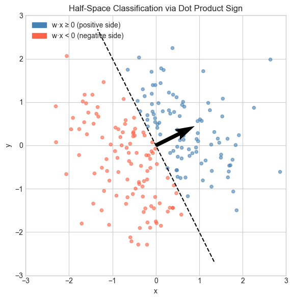
6. Experiments
# --- Experiment 1: Verify the formula numerically ---
# Hypothesis: algebraic dot product equals ||a||*||b||*cos(theta) for any vectors.
# Try changing: N_DIMS and the random seed.

np.random.seed(42)
N_DIMS = 5  # <-- modify this

a = np.random.randn(N_DIMS)
b = np.random.randn(N_DIMS)

algebraic  = np.dot(a, b)
geometric  = np.linalg.norm(a) * np.linalg.norm(b) * np.cos(angle_between(a, b))

print(f"Algebraic  a·b = {algebraic:.8f}")
print(f"Geometric  a·b = {geometric:.8f}")
print(f"Difference:     {abs(algebraic - geometric):.2e}  (floating point error only)")
Algebraic a·b = -0.67965499
Geometric a·b = -0.67965499
Difference: 0.00e+00 (floating point error only)
# --- Experiment 2: Cosine similarity vs raw dot product ---
# Hypothesis: two vectors pointing in the same direction have cosine sim = 1,
#             regardless of their magnitudes.
# Try changing: SCALE

a = np.array([1.0, 2.0, 3.0])
SCALE = 100.0  # <-- modify this
b = SCALE * a   # same direction, different magnitude

print(f"a = {a}")
print(f"b = SCALE * a = {b}")
print(f"Raw dot product:     {np.dot(a, b):.2f}  (grows with SCALE)")
print(f"Cosine similarity:   {cosine_similarity(a, b):.6f}  (always 1.0)")
print(f"Angle between them:  {angle_between(a, b, degrees=True):.6f}°  (always 0)")
# --- Experiment 3: Cosine similarity in NLP word space ---
# Simulate word embeddings. Find which word is most similar to a target.
# Try changing: TARGET_WORD and embedding dimension DIM.
np.random.seed(0)
words = ['cat', 'dog', 'fish', 'car', 'truck', 'road', 'kitten', 'puppy']
DIM = 10 # <-- modify this
# Random embeddings (in real NLP these are trained)
# Force 'cat' and 'kitten' to be similar
embeddings = {w: np.random.randn(DIM) for w in words}
embeddings['kitten'] = embeddings['cat'] + 0.3 * np.random.randn(DIM)
embeddings['puppy'] = embeddings['dog'] + 0.3 * np.random.randn(DIM)
TARGET_WORD = 'cat' # <-- modify this
target = embeddings[TARGET_WORD]
print(f"Most similar to '{TARGET_WORD}':")
sims = {w: cosine_similarity(target, v) for w, v in embeddings.items() if w != TARGET_WORD}
for w, s in sorted(sims.items(), key=lambda x: -x[1]):
print(f" {w:10s}: {s:.4f}")Most similar to 'cat':
kitten : 0.9568
puppy : 0.3760
dog : 0.3592
fish : 0.0649
truck : -0.0982
car : -0.4335
road : -0.7179
7. Exercises
Easy 1. Compute the angle between and using angle_between. Then verify geometrically. (Expected: 45 degrees)
Easy 2. Two vectors have magnitudes 3 and 5 and an angle of 60 degrees between them. What is their dot product? (Expected: compute from formula without knowing the components)
Medium 1. Write a function pairwise_cosine(X) that computes the full cosine similarity matrix for a batch of vectors (shape n×d). Use matrix operations only — no Python loops. (Hint: normalize rows first, then compute )
Medium 2. Plot the angle between two randomly generated vectors as you linearly interpolate one toward the other: for . How does the angle change — linearly, or not? (Hint: the angle is not a linear function of the interpolation parameter)
Hard. Prove that for unit vectors , we have . Use this to write an alternative angle computation that avoids arccos. When would this be numerically preferable? (Challenge: think about what happens near )
8. Mini Project — Semantic Search Engine
# --- Mini Project: Cosine Similarity Search ---
# Problem: Given a set of document embeddings and a query embedding,
#          return the top-k most similar documents using cosine similarity.
# Dataset: Synthetic 50-dimensional embeddings.
# Task: Implement the search function and analyze the angle distribution.

np.random.seed(123)
N_DOCS = 100
DIM    = 50
TOP_K  = 5

# Simulate document embeddings
doc_embeddings = np.random.randn(N_DOCS, DIM)

# Create a query as a noisy version of document 0
query_embedding = doc_embeddings[0] + 0.5 * np.random.randn(DIM)

doc_labels = [f'Document {i}' for i in range(N_DOCS)]

def semantic_search(query, documents, top_k=5):
    """
    Find top-k most similar documents to query using cosine similarity.

    Args:
        query:     array (d,)
        documents: array (n, d)
        top_k:     int

    Returns:
        indices: array (top_k,), indices of best matches
        scores:  array (top_k,), cosine similarity scores
    """
    # TODO 1: Normalize the query vector
    query_norm = None  # replace

    # TODO 2: Normalize each document vector (row-wise)
    doc_norms = None  # replace

    # TODO 3: Compute cosine similarities (dot products of normalized vectors)
    similarities = None  # replace, shape (n,)

    # TODO 4: Return top_k indices and scores
    top_indices = None  # replace
    return top_indices, similarities[top_indices]


# --- Test (uncomment after implementing) ---
# indices, scores = semantic_search(query_embedding, doc_embeddings, top_k=TOP_K)
# print(f"Query is a noisy version of Document 0.")
# print(f"Top {TOP_K} results:")
# for rank, (idx, score) in enumerate(zip(indices, scores)):
#     print(f"  Rank {rank+1}: {doc_labels[idx]} — similarity = {score:.4f}")

# --- Extension ---
# Compute all pairwise angles between documents.
# Plot a histogram of angles. What distribution do you expect in high dimensions?
# (Answer: angles concentrate near 90° — the curse of dimensionality from ch129.)
9. Chapter Summary & Connections
The geometric formula links the algebraic dot product to the angle between vectors.
Derivation uses the law of cosines applied to the triangle formed by , , and .
Cosine similarity is scale-invariant and lives in .
The sign of determines which side of a hyperplane lies on — the geometric core of linear classifiers.
Forward connections:
This reappears in ch133 — Angles Between Vectors, which applies this formula to measure orientation in any number of dimensions.
This reappears in ch134 — Projections: — the dot product divided by the squared norm.
This reappears in ch167 — Rotation via Matrices, where the cosine formula is encoded in rotation matrix entries.
Backward connection:
This deepens ch131 — Dot Product Intuition, replacing intuition with a precise derivation.
Going deeper: The formula generalizes to inner product spaces — abstract vector spaces with a notion of angle. This underpins Fourier analysis and quantum mechanics.