Prerequisites: ch132 (geometric dot product), ch112 (trigonometry), ch128 (norms)
You will learn:
How to compute the angle between vectors in any number of dimensions
How angles behave differently in high dimensions
Why measuring angles is more informative than measuring raw distance in some settings
Applications in data science: angular similarity, clustering, and orientation
Environment: Python 3.x, numpy, matplotlib
1. Concept
In 2D and 3D, the angle between two vectors is geometric and intuitive. In 100 dimensions, you cannot draw it — but the formula still works.
From ch132:
This computes a single angle between any two nonzero vectors, regardless of dimension.
Why angles matter beyond geometry: In high-dimensional data, distances are unreliable because all points tend to become equidistant (introduced in ch129). Angles are more stable. Two word embeddings may be far apart in L2 distance but have a small angle — meaning they represent similar concepts. Cosine similarity exploits this.
Common misconceptions:
The angle formula gives . You cannot get a 270-degree angle between two vectors — rotation sense has no meaning here.
Orthogonality () does not mean the vectors are geometrically perpendicular in any visual sense in high dimensions. It means they share no information.
2. Intuition & Mental Models
Geometric: Think of shining a flashlight (vector ) and a second beam (). The angle between them is what you’d measure with a protractor at the source. In higher dimensions, you cannot visualize this, but the dot product formula gives the same measurement.
Information-theoretic: Two vectors at a small angle encode nearly the same directional information. Two vectors at 90° are maximally uninformative about each other. Two at 180° are perfectly opposite. The angle is a measure of directional agreement.
Computational: For machine learning, the angle formula is used to measure how similar two high-dimensional feature vectors are. arccos(dot(a,b) / (norm(a)*norm(b))) is a one-liner for angles in .
Recall from ch132 that cosine similarity = . The angle is simply the inverse cosine of that.
3. Visualization
# --- Visualization: Angle between vectors in 2D and 3D ---

import numpy as np
import matplotlib.pyplot as plt
from mpl_toolkits.mplot3d import Axes3D

plt.style.use('seaborn-v0_8-whitegrid')

def angle_between(a, b, degrees=True):
    a, b = np.asarray(a, float), np.asarray(b, float)
    cos_t = np.clip(np.dot(a, b) / (np.linalg.norm(a) * np.linalg.norm(b)), -1, 1)
    theta = np.arccos(cos_t)
    return np.degrees(theta) if degrees else theta

fig = plt.figure(figsize=(12, 5))

# 2D case
ax2 = fig.add_subplot(121)
a2 = np.array([2.0, 1.0])
b2 = np.array([0.5, 2.0])
ax2.quiver(0, 0, a2[0], a2[1], angles='xy', scale_units='xy', scale=1, color='steelblue')
ax2.quiver(0, 0, b2[0], b2[1], angles='xy', scale_units='xy', scale=1, color='tomato')
angle2d = angle_between(a2, b2)
ax2.set_xlim(-0.5, 3); ax2.set_ylim(-0.5, 3)
ax2.set_aspect('equal')
ax2.set_title(f'2D: θ = {angle2d:.1f}°')
ax2.set_xlabel('x'); ax2.set_ylabel('y')
ax2.text(1.5, 0.2, f'a = {a2}', color='steelblue')
ax2.text(0.1, 1.8, f'b = {b2}', color='tomato')

# 3D case
ax3 = fig.add_subplot(122, projection='3d')
a3 = np.array([1.0, 1.0, 0.0])
b3 = np.array([0.0, 1.0, 1.0])
ax3.quiver(0, 0, 0, a3[0], a3[1], a3[2], color='steelblue', linewidth=2)
ax3.quiver(0, 0, 0, b3[0], b3[1], b3[2], color='tomato',    linewidth=2)
angle3d = angle_between(a3, b3)
ax3.set_xlim(0, 1.2); ax3.set_ylim(0, 1.2); ax3.set_zlim(0, 1.2)
ax3.set_title(f'3D: θ = {angle3d:.1f}°')
ax3.set_xlabel('x'); ax3.set_ylabel('y'); ax3.set_zlabel('z')

plt.suptitle('Angle Formula Works in Any Dimension', fontsize=13, fontweight='bold')
plt.tight_layout()
plt.show()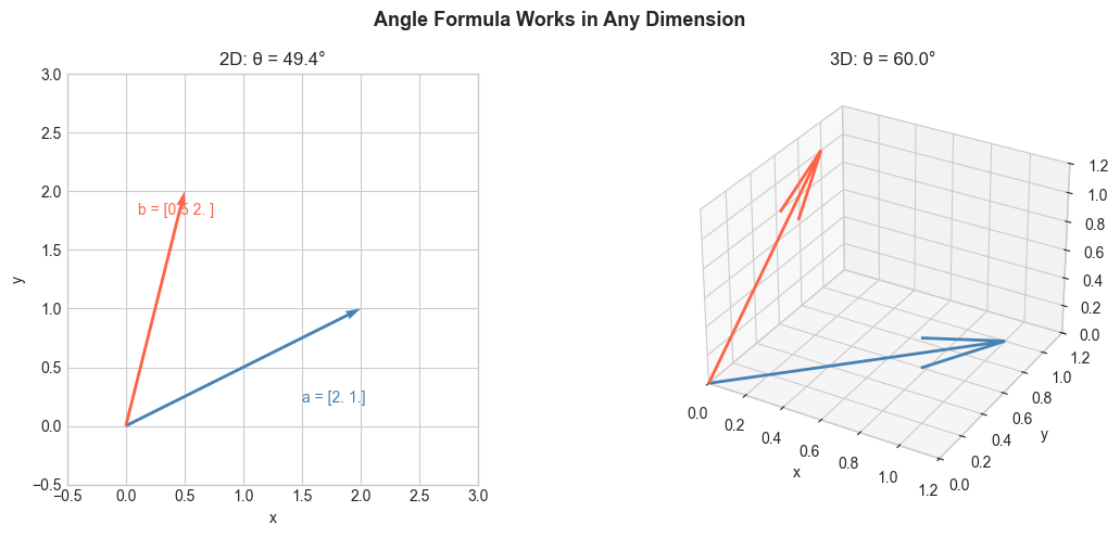
# --- Visualization: Angle distribution of random vectors in high dimensions ---
# Key phenomenon: in high dimensions, most random vectors are near-orthogonal.

N_SAMPLES = 3000
dimensions = [2, 5, 20, 100, 500]

fig, axes = plt.subplots(1, len(dimensions), figsize=(16, 4), sharey=True)

for ax, dim in zip(axes, dimensions):
    # Generate random unit vectors
    vecs = np.random.randn(N_SAMPLES, dim)
    vecs /= np.linalg.norm(vecs, axis=1, keepdims=True)

    # Compute angles between consecutive pairs
    a_batch = vecs[:N_SAMPLES//2]
    b_batch = vecs[N_SAMPLES//2:]
    dots = np.sum(a_batch * b_batch, axis=1)
    angles = np.degrees(np.arccos(np.clip(dots, -1, 1)))

    ax.hist(angles, bins=40, color='steelblue', edgecolor='white', alpha=0.85)
    ax.axvline(90, color='red', linestyle='--', linewidth=1.2, label='90°')
    ax.set_title(f'd = {dim}\nμ = {angles.mean():.1f}°\nσ = {angles.std():.1f}°', fontsize=9)
    ax.set_xlabel('Angle (°)')
    ax.set_xlim(0, 180)

axes[0].set_ylabel('Count')
plt.suptitle('Distribution of Angles Between Random Unit Vectors by Dimension',
             fontsize=12, fontweight='bold')
plt.tight_layout()
plt.show()

print("As dimension grows, angles concentrate near 90°.")
print("Most random high-dimensional vectors are nearly orthogonal.")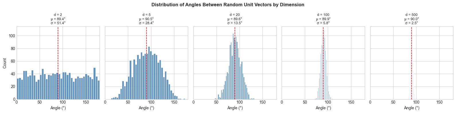
As dimension grows, angles concentrate near 90°.
Most random high-dimensional vectors are nearly orthogonal.
4. Mathematical Formulation
The angle formula (from ch132):
Key angle values and what they mean:
| Interpretation | ||
|---|---|---|
| 1 | Identical direction | |
| Partially aligned | ||
| 0 | Orthogonal (no alignment) | |
| Partially opposing | ||
| -1 | Exactly opposite |
Angular distance as a metric:
This is a proper distance metric on the unit sphere, satisfying: non-negativity, symmetry, and the triangle inequality.
Standard basis angles: The angle between standard basis vector and any vector is:
These are called the direction cosines of . They satisfy: .
5. Python Implementation
# --- Implementation: Angles, direction cosines, angular distance ---

def angle_between(a, b, degrees=True):
    """
    Angle between two non-zero vectors in any dimension.

    Args:
        a, b:    array-like, shape (n,)
        degrees: if True, return degrees; else radians

    Returns:
        float in [0, 180] degrees or [0, π] radians
    """
    a, b = np.asarray(a, float), np.asarray(b, float)
    cos_theta = np.clip(np.dot(a, b) / (np.linalg.norm(a) * np.linalg.norm(b)), -1.0, 1.0)
    theta = np.arccos(cos_theta)
    return np.degrees(theta) if degrees else theta


def direction_cosines(v):
    """
    Direction cosines: angles that v makes with each standard basis vector.

    Args:
        v: array-like, shape (n,)

    Returns:
        angles_deg: array (n,), angles in degrees with each axis
    """
    v = np.asarray(v, float)
    v_hat = v / np.linalg.norm(v)
    cos_angles = v_hat  # cos(theta_i) = v_i / ||v||, which equals v_hat_i
    return np.degrees(np.arccos(np.clip(cos_angles, -1, 1)))


def angular_distance(a, b):
    """
    Normalized angular distance in [0, 1].
    0 = identical direction, 1 = opposite direction.

    Args:
        a, b: array-like, shape (n,)

    Returns:
        float in [0, 1]
    """
    return angle_between(a, b, degrees=False) / np.pi


# Tests
v = np.array([1.0, 1.0, 0.0])
print("Direction cosines of [1, 1, 0]:")
dc = direction_cosines(v)
for i, angle in enumerate(dc):
    print(f"  With e_{i+1}: {angle:.1f}°")
print(f"  Sum of cos²(θ_i): {np.sum(np.cos(np.radians(dc))**2):.6f}  (should be 1.0)")

print()
print(f"Angular distance [1,0] vs [0,1]:  {angular_distance([1,0],[0,1]):.3f}  (expect 0.5)")
print(f"Angular distance [1,0] vs [-1,0]: {angular_distance([1,0],[-1,0]):.3f}  (expect 1.0)")
print(f"Angular distance [1,0] vs [1,0]:  {angular_distance([1,0],[1,0]):.3f}  (expect 0.0)")
Direction cosines of [1, 1, 0]:
With e_1: 45.0°
With e_2: 45.0°
With e_3: 90.0°
Sum of cos²(θ_i): 1.000000 (should be 1.0)
Angular distance [1,0] vs [0,1]: 0.500 (expect 0.5)
Angular distance [1,0] vs [-1,0]: 1.000 (expect 1.0)
Angular distance [1,0] vs [1,0]: 0.000 (expect 0.0)
6. Experiments
# --- Experiment 1: Angle concentration in high dimensions ---
# Hypothesis: as dimension increases, the std of pairwise angles shrinks.
# This means high-dimensional random vectors become "indistinguishably orthogonal".
# Try changing: N_PAIRS

N_PAIRS = 2000  # <-- modify this
dims = [2, 5, 10, 20, 50, 100, 200, 500]

mean_angles = []
std_angles  = []

for d in dims:
    a_batch = np.random.randn(N_PAIRS, d)
    b_batch = np.random.randn(N_PAIRS, d)
    a_batch /= np.linalg.norm(a_batch, axis=1, keepdims=True)
    b_batch /= np.linalg.norm(b_batch, axis=1, keepdims=True)
    dots = np.sum(a_batch * b_batch, axis=1)
    angles = np.degrees(np.arccos(np.clip(dots, -1, 1)))
    mean_angles.append(angles.mean())
    std_angles.append(angles.std())

fig, axes = plt.subplots(1, 2, figsize=(12, 4))
axes[0].semilogx(dims, mean_angles, 'o-', color='steelblue')
axes[0].axhline(90, color='gray', linestyle='--', alpha=0.5)
axes[0].set_xlabel('Dimension (log scale)'); axes[0].set_ylabel('Mean angle (°)')
axes[0].set_title('Mean Angle Converges to 90°')

axes[1].semilogx(dims, std_angles, 'o-', color='tomato')
axes[1].set_xlabel('Dimension (log scale)'); axes[1].set_ylabel('Std of angles (°)')
axes[1].set_title('Angle Distribution Narrows (Concentration)')

plt.tight_layout()
plt.show()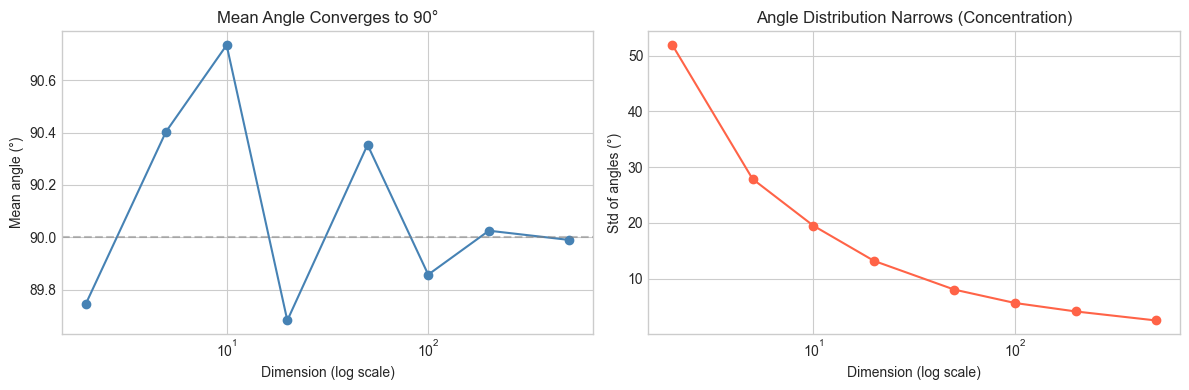
# --- Experiment 2: Angle vs L2 distance for classification ---
# Hypothesis: angle-based similarity better captures direction than L2 distance.
# Vectors of different magnitudes but same direction should be "similar".
# Try changing: SCALE

SCALE = 10.0  # <-- modify this (scales one class of vectors)

np.random.seed(42)
# Class A: vectors near [1, 0]
# Class B: vectors near [0, 1]
class_a = np.random.randn(50, 2) * 0.3 + np.array([1.0, 0.0])
class_b = np.random.randn(50, 2) * 0.3 + np.array([0.0, 1.0])

# Scale class A vectors — same direction, different magnitude
class_a_scaled = class_a * SCALE

query = np.array([0.8, 0.1])  # should be similar to class A

# L2 distances
l2_a = np.mean(np.linalg.norm(class_a_scaled - query, axis=1))
l2_b = np.mean(np.linalg.norm(class_b           - query, axis=1))

# Cosine similarities
def batch_cosine_sim(X, q):
    X_n = X / np.linalg.norm(X, axis=1, keepdims=True)
    q_n = q / np.linalg.norm(q)
    return X_n @ q_n

cos_a = np.mean(batch_cosine_sim(class_a_scaled, query))
cos_b = np.mean(batch_cosine_sim(class_b, query))

print(f"SCALE = {SCALE}")
print(f"\nL2 distance to class A (scaled): {l2_a:.2f}")
print(f"L2 distance to class B:          {l2_b:.2f}")
print(f"→ L2 says: query is closer to {'A' if l2_a < l2_b else 'B'}")
print(f"\nCosine similarity to class A: {cos_a:.4f}")
print(f"Cosine similarity to class B: {cos_b:.4f}")
print(f"→ Cosine says: query is closer to {'A' if cos_a > cos_b else 'B'}")
print("\nL2 is fooled by scale; cosine is not.")
SCALE = 10.0
L2 distance to class A (scaled): 9.27
L2 distance to class B: 1.29
→ L2 says: query is closer to B
Cosine similarity to class A: 0.9437
Cosine similarity to class B: 0.0934
→ Cosine says: query is closer to A
L2 is fooled by scale; cosine is not.
7. Exercises
Easy 1. Compute the angle between and . (Expected: 90° — verify they are orthogonal via dot product)
Easy 2. What is the angle between any vector and its own negative? What does this mean geometrically? (Expected: 180°)
Medium 1. Write a function all_angles(V) that takes an matrix of unit vectors and returns the full angle matrix (in degrees). Use vectorized operations — no Python loops. (Hint: the dot product matrix is V @ V.T, then arccos)
Medium 2. Plot the angle between and a vector that rotates from to in 1000 steps. Compare this to the cosine similarity over the same path. Which is more linear in the rotation angle? (This matters for interpolation — see ch105 Interpolation and Splines)
Hard. In dimension , the expected angle between two random unit vectors is exactly for all . But the variance shrinks as grows. Derive an approximation for the standard deviation of pairwise angles as a function of . Verify numerically. (Challenge: use the central limit theorem — the dot product is a sum of i.i.d. terms)
8. Mini Project — Angular Clustering
# --- Mini Project: Angular Nearest-Neighbor Classifier ---
# Problem: Classify 2D data points using angular distance to class centroids.
# Unlike Euclidean k-nearest-neighbors, this classifier is scale-invariant.
# Dataset: Three classes of direction-based clusters in 2D.
# Task: Implement angular_classify and compare accuracy to L2 classification.

np.random.seed(0)

# Three direction-based classes (different magnitudes, similar directions)
class_directions = [np.array([1.0, 0.0]),
                     np.array([0.0, 1.0]),
                     np.array([-1.0, -1.0]) / np.sqrt(2)]
class_labels = ['East', 'North', 'Southwest']

# Generate points: each class has different magnitudes (noise in scale)
X_train = []
y_train = []
for label, direction in enumerate(class_directions):
    magnitudes = np.random.uniform(0.5, 5.0, 30)  # variable magnitude
    noise = np.random.randn(30, 2) * 0.15          # small angle noise
    points = magnitudes[:, None] * direction + noise
    X_train.extend(points)
    y_train.extend([label] * 30)

X_train = np.array(X_train)
y_train = np.array(y_train)

# Compute class centroids
centroids = np.array([X_train[y_train == c].mean(axis=0) for c in range(3)])

def angular_classify(X, centroids):
    """
    Classify each point in X by finding the centroid with smallest angular distance.

    Args:
        X:         array (n, d) — points to classify
        centroids: array (k, d) — class centroids

    Returns:
        labels: array (n,), predicted class indices
    """
    # TODO: normalize X and centroids
    # TODO: compute cosine similarity matrix (n x k)
    # TODO: return argmax of similarity for each point
    pass

def l2_classify(X, centroids):
    """
    Classify each point by L2 distance to centroids.
    """
    # TODO: compute distance from each point to each centroid, return argmin
    pass

# --- Evaluate (uncomment after implementing) ---
# pred_angular = angular_classify(X_train, centroids)
# pred_l2      = l2_classify(X_train, centroids)
# acc_angular  = np.mean(pred_angular == y_train)
# acc_l2       = np.mean(pred_l2      == y_train)
# print(f"Angular classifier accuracy: {acc_angular:.2%}")
# print(f"L2 classifier accuracy:      {acc_l2:.2%}")

# --- Visualize ---
# Plot X_train colored by true class, with class centroids marked.
# Visually verify that angle-based separation is clean despite magnitude variation.
9. Chapter Summary & Connections
The angle works in any dimension.
In high dimensions, random vectors concentrate near — most pairs become nearly orthogonal.
Angle-based similarity is scale-invariant; L2 distance is not. This makes angles preferable for directional comparisons.
Direction cosines decompose a vector into its angular relationships with each axis.
Forward connections:
This reappears in ch134 — Projections, where the angle formula gives the length of the shadow: .
This reappears in ch135 — Orthogonality, which formalizes what means structurally.
This reappears in ch183 — PCA Intuition, where orthogonal directions of maximum variance are found.
Backward connection:
This applies the derivation from ch132 — Geometric Meaning of Dot Product, which proved .
Going deeper: The angle formula on the unit sphere defines the geodesic distance on . Spherical geometry and spherical harmonics build on this foundation.