Prerequisites: ch131 (dot product), ch132 (geometric dot product), ch130 (direction vectors)
You will learn:
How to project one vector onto another
The decomposition of a vector into parallel and perpendicular components
Why projection is the foundation of least squares, PCA, and Gram-Schmidt
How to build orthogonal decomposition computationally
Environment: Python 3.x, numpy, matplotlib
1. Concept
Given two vectors and , the projection of onto is the vector along that is closest to .
Think of shining a light directly perpendicular to and casting the shadow of onto the line containing . The shadow is the projection.
Every vector can be split into exactly two pieces:
Common misconceptions:
The projection of onto is a vector in the direction of , not .
Projection is not symmetric: in general.
The component (scalar projection) and the projection (vector) are different things. One is a number, one is a vector.
2. Intuition & Mental Models
Physical: A hill casts a shadow on the ground. The length of the shadow depends on the angle of the sun. The shadow is the projection of the hill’s height vector onto the ground plane.
Work in physics: If you push a box with force but the box can only move in direction , only the component of along does work. That component is the scalar projection.
Computational: Projection answers the question: given a vector, how much of it lies along a particular axis? This is how PCA extracts principal components (ch182): it projects data onto the direction of maximum variance.
Least squares connection: The best-fit line through data points is the one whose residuals (errors) are perpendicular to the line. The fitted values are projections of the data onto the line’s direction. (ch199 — Linear Regression via Matrix Algebra)
Recall from ch132: . The scalar projection is exactly — the dot product with the unit vector in 's direction.
3. Visualization
# --- Visualization: Vector projection and decomposition ---

import numpy as np
import matplotlib.pyplot as plt

plt.style.use('seaborn-v0_8-whitegrid')

def proj(a, b):
    """Project vector a onto vector b."""
    b_hat = b / np.linalg.norm(b)
    return np.dot(a, b_hat) * b_hat

a = np.array([3.0, 2.5])
b = np.array([4.0, 1.0])

p = proj(a, b)        # vector projection
e = a - p             # perpendicular component

fig, ax = plt.subplots(figsize=(8, 6))

ORIGIN = np.zeros(2)

# Draw b extended as a line
b_hat = b / np.linalg.norm(b)
t = np.linspace(-0.5, 5, 100)
ax.plot(t * b_hat[0], t * b_hat[1], 'gray', linestyle='--', linewidth=1, label='Line of b')

# Draw vectors
kw = dict(angles='xy', scale_units='xy', scale=1, width=0.012)
ax.quiver(*ORIGIN, *a, color='steelblue', **kw, label=f'a = {a}')
ax.quiver(*ORIGIN, *b, color='dimgray',   **kw, label=f'b = {b}')
ax.quiver(*ORIGIN, *p, color='tomato',    **kw, label=f'proj_b(a) = [{p[0]:.2f}, {p[1]:.2f}]')
ax.quiver(*p,      *e, color='seagreen',  **kw, label=f'perp = a - proj_b(a)')

# Right-angle mark at foot of perpendicular
size = 0.15
b_dir = b_hat
perp_dir = np.array([-b_dir[1], b_dir[0]])
corner = p + size * perp_dir
ax.plot([p[0], corner[0], corner[0] + size*b_dir[0]],
         [p[1], corner[1], corner[1] + size*b_dir[1]], 'k-', linewidth=1)

ax.set_xlim(-0.5, 5); ax.set_ylim(-0.5, 3.5)
ax.set_aspect('equal')
ax.legend(fontsize=9, loc='upper left')
ax.set_title('Vector Projection: a = proj_b(a) + perpendicular')
ax.set_xlabel('x'); ax.set_ylabel('y')
plt.tight_layout()
plt.show()

print(f"Verification: proj + perp = a?")
print(f"  p + e = {p + e}  vs  a = {a}")
print(f"  Perp is orthogonal to b: {np.isclose(np.dot(e, b), 0)}")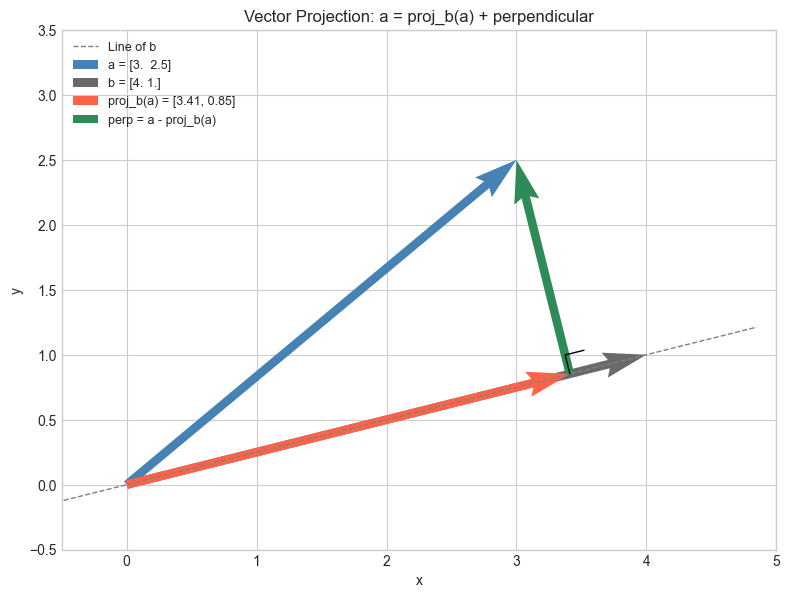
Verification: proj + perp = a?
  p + e = [3.  2.5]  vs  a = [3.  2.5]
  Perp is orthogonal to b: True
# --- Visualization: Projection onto multiple axes ---
# Project a 2D vector onto the standard basis vectors and several others.
# Shows how projection extracts components.

a = np.array([2.0, 3.0])
axes_to_project = [
    (np.array([1.0, 0.0]),  'e1 (x-axis)'),
    (np.array([0.0, 1.0]),  'e2 (y-axis)'),
    (np.array([1.0, 1.0]),  'diagonal [1,1]'),
    (np.array([1.0, -1.0]), 'diagonal [1,-1]'),
]

fig, axes = plt.subplots(2, 2, figsize=(10, 8))
for ax, (b_vec, label) in zip(axes.flat, axes_to_project):
    p = proj(a, b_vec)
    e = a - p
    scalar_proj = np.dot(a, b_vec / np.linalg.norm(b_vec))

    b_hat = b_vec / np.linalg.norm(b_vec)
    t = np.linspace(-4, 4, 100)
    ax.plot(t * b_hat[0], t * b_hat[1], 'gray', linestyle='--', linewidth=0.8)

    kw = dict(angles='xy', scale_units='xy', scale=1, width=0.015)
    ax.quiver(0, 0, a[0], a[1],   color='steelblue', **kw)
    ax.quiver(0, 0, p[0], p[1],   color='tomato',    **kw)
    ax.quiver(p[0], p[1], e[0], e[1], color='seagreen', **kw)

    ax.set_xlim(-4, 4); ax.set_ylim(-4, 4)
    ax.set_aspect('equal')
    ax.axhline(0, color='gray', linewidth=0.4)
    ax.axvline(0, color='gray', linewidth=0.4)
    ax.set_title(f'Projection onto {label}\nScalar proj = {scalar_proj:.2f}', fontsize=9)

plt.suptitle('Projecting a = [2, 3] onto Different Directions', fontsize=12, fontweight='bold')
plt.tight_layout()
plt.show()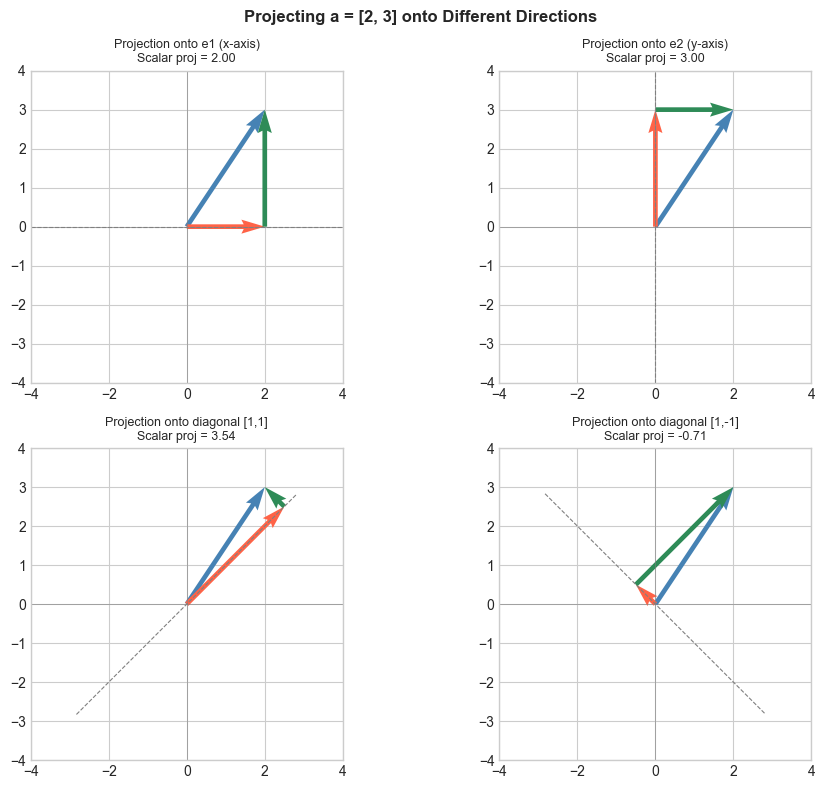
4. Mathematical Formulation
Scalar projection (a number — the signed length of the shadow):
Vector projection (a vector — the shadow itself):
Written using the unit vector :
Orthogonal decomposition:
Verification: The remainder satisfies :
Projection matrix (projects any vector onto the direction):
Then . (This connects to ch168 — Projection Matrices in linear algebra.)
5. Python Implementation
# --- Implementation: scalar_proj, vector_proj, orthogonal_decompose ---

def scalar_proj(a, b):
    """
    Scalar projection of a onto b (signed length of shadow).

    Args:
        a, b: array-like, shape (n,)

    Returns:
        float: can be negative if angle > 90°
    """
    a, b = np.asarray(a, float), np.asarray(b, float)
    return np.dot(a, b) / np.linalg.norm(b)


def vector_proj(a, b):
    """
    Vector projection of a onto b.

    Args:
        a, b: array-like, shape (n,)

    Returns:
        array, shape (n,): vector in direction of b
    """
    a, b = np.asarray(a, float), np.asarray(b, float)
    return (np.dot(a, b) / np.dot(b, b)) * b


def orthogonal_decompose(a, b):
    """
    Decompose a into components parallel and perpendicular to b.

    Args:
        a, b: array-like, shape (n,)

    Returns:
        parallel:  array (n,), component along b
        perp:      array (n,), component perpendicular to b
    """
    parallel = vector_proj(a, b)
    perp = np.asarray(a, float) - parallel
    return parallel, perp


def projection_matrix(b):
    """
    Build the projection matrix P = b_hat @ b_hat.T.
    Applying P to any vector projects it onto the b direction.

    Args:
        b: array-like, shape (n,)

    Returns:
        P: array (n, n)
    """
    b = np.asarray(b, float)
    b_hat = b / np.linalg.norm(b)
    return np.outer(b_hat, b_hat)  # outer product = b_hat @ b_hat.T


# Tests
a = np.array([3.0, 4.0])
b = np.array([1.0, 0.0])  # x-axis

print(f"scalar_proj({a}, {b}) = {scalar_proj(a, b):.2f}  (expect 3.0 — x-component)")
print(f"vector_proj({a}, {b}) = {vector_proj(a, b)}  (expect [3, 0])")

par, perp = orthogonal_decompose(a, b)
print(f"\nParallel:     {par}")
print(f"Perpendicular:{perp}")
print(f"Reconstructs: {par + perp}  (should equal a = {a})")
print(f"Perp · b = {np.dot(perp, b):.2e}  (should be ~0)")

# Projection matrix test
b2 = np.array([1.0, 1.0])
P = projection_matrix(b2)
print(f"\nProjection matrix onto [1,1]:")
print(P)
print(f"P @ a = {P @ a}  vs  vector_proj(a, b2) = {vector_proj(a, b2)}")
scalar_proj([3. 4.], [1. 0.]) = 3.00 (expect 3.0 — x-component)
vector_proj([3. 4.], [1. 0.]) = [3. 0.] (expect [3, 0])
Parallel: [3. 0.]
Perpendicular:[0. 4.]
Reconstructs: [3. 4.] (should equal a = [3. 4.])
Perp · b = 0.00e+00 (should be ~0)
Projection matrix onto [1,1]:
[[0.5 0.5]
[0.5 0.5]]
P @ a = [3.5 3.5] vs vector_proj(a, b2) = [3.5 3.5]
6. Experiments
# --- Experiment 1: Projection idempotency ---
# Hypothesis: projecting a projection gives the same projection.
# P^2 = P (projection matrices are idempotent).
# Try changing: b

b = np.array([3.0, 1.0])  # <-- modify this
a = np.array([2.0, 5.0])

proj_once  = vector_proj(a, b)
proj_twice = vector_proj(proj_once, b)

print(f"proj(a, b)         = {proj_once}")
print(f"proj(proj(a,b), b) = {proj_twice}")
print(f"Equal: {np.allclose(proj_once, proj_twice)}")
print("Projecting an already-projected vector changes nothing.")
proj(a, b) = [3.3 1.1]
proj(proj(a,b), b) = [3.3 1.1]
Equal: True
Projecting an already-projected vector changes nothing.
# --- Experiment 2: Closest point on a line to a given point ---
# The projection of a point onto a line is the closest point on that line.
# Try changing: QUERY_POINT and LINE_DIR

LINE_POINT = np.array([1.0, 1.0])  # a point the line passes through
LINE_DIR   = np.array([2.0, 1.0])  # direction of the line
QUERY_POINT = np.array([4.0, 3.0])  # <-- modify this

# Translate to origin: vector from line point to query
v = QUERY_POINT - LINE_POINT
# Project v onto line direction
v_proj = vector_proj(v, LINE_DIR)
# Closest point on line
closest = LINE_POINT + v_proj

dist = np.linalg.norm(QUERY_POINT - closest)

# Visualize
fig, ax = plt.subplots(figsize=(7, 6))
t = np.linspace(-2, 4, 100)
line_hat = LINE_DIR / np.linalg.norm(LINE_DIR)
ax.plot(LINE_POINT[0] + t*line_hat[0], LINE_POINT[1] + t*line_hat[1],
         'gray', linestyle='--', label='Line')
ax.plot(*QUERY_POINT, 'o', color='steelblue', markersize=10, label='Query point')
ax.plot(*closest,     's', color='tomato',    markersize=10, label='Closest point (projection)')
ax.plot([QUERY_POINT[0], closest[0]], [QUERY_POINT[1], closest[1]],
         'seagreen', linestyle=':', linewidth=2, label=f'Distance = {dist:.3f}')
ax.set_aspect('equal')
ax.legend(fontsize=9)
ax.set_title('Closest Point on Line via Projection')
ax.set_xlabel('x'); ax.set_ylabel('y')
plt.tight_layout()
plt.show()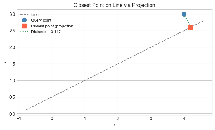
# --- Experiment 3: Projection and least-squares ---
# Project noisy data onto a line y = mx through the origin.
# The slope m that minimizes total squared distance is found via projection.
# Try changing: TRUE_SLOPE and NOISE_LEVEL

np.random.seed(99)
TRUE_SLOPE  = 2.0   # <-- modify this
NOISE_LEVEL = 0.8   # <-- modify this
N = 30

x = np.linspace(0, 3, N)
y = TRUE_SLOPE * x + NOISE_LEVEL * np.random.randn(N)

# Data vector and "model vector" direction
data_vec  = y                          # observed y values
model_dir = x                          # x values as direction vector

# Scalar projection gives the best slope (least squares through origin)
m_hat = np.dot(data_vec, model_dir) / np.dot(model_dir, model_dir)

fig, ax = plt.subplots(figsize=(8, 5))
ax.scatter(x, y, color='steelblue', label='Data')
ax.plot(x, TRUE_SLOPE * x, 'gray', linestyle='--', label=f'True slope = {TRUE_SLOPE}')
ax.plot(x, m_hat * x, 'tomato', linewidth=2, label=f'Projected slope = {m_hat:.3f}')
ax.set_xlabel('x'); ax.set_ylabel('y')
ax.set_title('Least-Squares via Projection')
ax.legend()
plt.tight_layout()
plt.show()

print(f"True slope:      {TRUE_SLOPE}")
print(f"Projected slope: {m_hat:.4f}")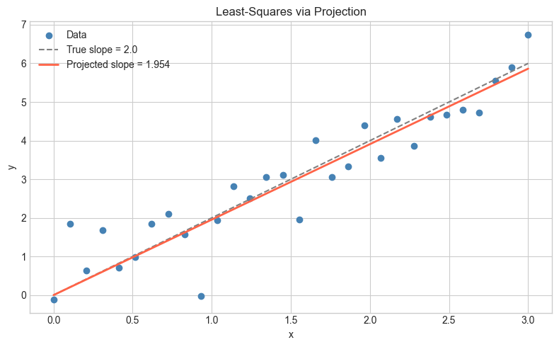
True slope:      2.0
Projected slope: 1.9544
7. Exercises
Easy 1. Project onto . Then project onto . What do you get, and why? (Expected: the and components of )
Easy 2. Compute both the scalar and vector projection of onto . (Expected: scalar = , vector = )
Medium 1. Write a function closest_point_on_line(p, line_point, line_dir) that returns the closest point on an infinite line to point . Test it on several cases and verify the distance is minimized. (Hint: use vector_proj on the translated vector)
Medium 2. Show numerically that for a randomly generated projection matrix (where ). Also compute (the complementary projection) and verify that .
Hard. Given points and a direction unit vector , show that the slope that minimizes (sum of squared perpendicular distances) is given by the direction of the eigenvector of the data covariance matrix. (This is the geometric core of PCA — ch182)
8. Mini Project — Signal Decomposition
# --- Mini Project: Signal Decomposition via Projection ---
# Problem: Decompose a noisy time-series signal into a smooth trend component
#          and a noise component using projection.
# Dataset: Synthetic signal = polynomial trend + noise.
# Task: Complete the project_signal function and visualize the decomposition.

np.random.seed(5)
N = 100
t = np.linspace(0, 2*np.pi, N)

# True trend: linear combination of a few basis vectors
signal = 2.0 * np.sin(t) + 0.5 * np.cos(2*t) + 0.3 * np.random.randn(N)

# Basis vectors for smooth component (low-frequency)
basis_1 = np.sin(t)
basis_2 = np.cos(t)

def project_signal(signal, basis_vectors):
    """
    Project signal onto the subspace spanned by basis_vectors.

    Assumes basis vectors are ORTHOGONAL (not orthonormal).

    Args:
        signal:        array (N,)
        basis_vectors: list of arrays, each shape (N,)

    Returns:
        projection: array (N,), smooth component
        residual:   array (N,), noise component
    """
    projection = np.zeros_like(signal)
    for basis in basis_vectors:
        # TODO: add the projection of signal onto this basis vector
        projection += None  # replace with vector_proj(signal, basis)

    residual = signal - projection
    return projection, residual


# --- Test (uncomment after implementing) ---
# smooth, noise = project_signal(signal, [basis_1, basis_2])
#
# fig, axes = plt.subplots(3, 1, figsize=(10, 8), sharex=True)
# axes[0].plot(t, signal,  color='steelblue', label='Noisy signal')
# axes[0].set_title('Original Signal')
# axes[1].plot(t, smooth,  color='tomato',    label='Smooth component (projection)')
# axes[1].set_title('Smooth Component (Projected onto sin, cos)')
# axes[2].plot(t, noise,   color='seagreen',  label='Residual (noise)')
# axes[2].set_title('Residual = Noise')
# for ax in axes:
#     ax.legend(); ax.set_ylabel('Amplitude')
# axes[-1].set_xlabel('t')
# plt.tight_layout()
# plt.show()
#
# print(f"Smooth component energy: {np.dot(smooth, smooth):.2f}")
# print(f"Noise component energy:  {np.dot(noise, noise):.2f}")
# print(f"Smooth ⊥ Noise: {np.isclose(np.dot(smooth, noise), 0, atol=1e-8)}")

# --- Extension ---
# Add basis_3 = np.cos(2*t) to the basis. Does the smooth component improve?
# This is the idea behind Fourier analysis — projecting onto sine/cosine bases.
9. Chapter Summary & Connections
Vector projection: — the component of along .
Orthogonal decomposition: every vector splits into a parallel part (projection) and a perpendicular remainder, and these two parts are orthogonal.
The projection matrix is idempotent: .
The closest point on a line to any external point is its projection — the perpendicular foot.
Forward connections:
This reappears in ch135 — Orthogonality, where we formalize the perpendicular component and build orthogonal bases.
This reappears in ch168 — Projection Matrices, where generalizes projection to subspaces.
This is the geometric core of ch199 — Linear Regression via Matrix Algebra: the fitted values are projections of onto the column space of .
This reappears in ch182 — PCA Intuition: PCA finds the directions that maximize projected variance.
Backward connection:
This builds directly on ch132 — Geometric Meaning of Dot Product: scalar projection .
Going deeper: Gram-Schmidt orthogonalization (ch170) applies projection iteratively to build a complete orthogonal basis from any set of independent vectors. Projection onto subspaces is the foundation of QR decomposition.