Prerequisites: ch141 (Linear Independence), ch139 (Basis and Dimension), ch135 (Orthogonality), ch124 (Vector Representation)
You will learn:
How a basis defines a coordinate system and why coordinates depend on the chosen basis
How to convert vectors between different coordinate systems
Orthonormal, oblique, and polar coordinate systems — and when each is useful
How change of basis is used in signal processing, graphics, and ML
The computational cost and numerical stability trade-offs of coordinate choices
Environment: Python 3.x, numpy, matplotlib
1. Concept
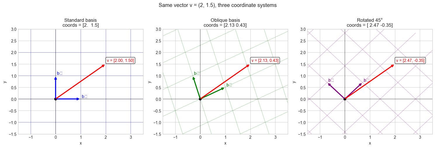
A coordinate system is a way to assign a unique label (a tuple of numbers) to every point in a space. Every coordinate system for a vector space V is defined by a basis B = {b₁, ..., bₙ}: the coordinates of a vector v are the scalars (c₁, ..., cₙ) such that v = c₁b₁ + ... + cₙbₙ.
The same physical vector has different coordinates in different coordinate systems — but the vector itself is unchanged. Coordinate systems are bookkeeping, not substance.
Why coordinate systems matter:
Computation happens in coordinates. Choosing the right coordinate system makes computations simpler, faster, or more numerically stable.
In graphics and robotics, different objects (camera, world, robot arm) have their own coordinate frames, and transforming between them is a fundamental operation.
In ML, feature spaces are coordinate systems. PCA finds a new coordinate system where variance is maximized along axes — the same data, re-expressed.
Common misconception: “The standard (Cartesian) coordinate system is special.” For computation, it is merely convenient. Many problems are simpler in non-standard coordinates: Fourier analysis works in a frequency coordinate system; PCA works in a variance-aligned coordinate system.
2. Intuition & Mental Models
Geometric model: Think of a coordinate system as a grid drawn on space. The standard grid has perpendicular lines spaced 1 unit apart. A non-standard basis draws a different grid — perhaps slanted, perhaps with different spacing. Any point lies at a unique grid intersection, but the grid address changes when the grid changes.
Computational model: Think of coordinates as the output of a measurement device. Each basis vector is one sensor. The sensor reads how much of the signal is aligned with its direction. Change the sensors, and the readings change — even though the signal (the vector) is the same.
Recall from ch139 (Basis and Dimension): every basis provides unique coordinates. Recall from ch141 (Linear Independence): independence is what makes coordinates unique — dependent bases give ambiguous readings.
Physical analogy: GPS coordinates and city addresses both locate the same place, but in different coordinate systems. Converting between them requires knowing the relationship between the two systems — this is the change-of-basis matrix.
3. Visualization
# --- Visualization: Same vector in three different coordinate systems ---

import numpy as np
import matplotlib.pyplot as plt

plt.style.use('seaborn-v0_8-whitegrid')

fig, axes = plt.subplots(1, 3, figsize=(15, 5))

v = np.array([2.0, 1.5])  # the actual vector — same in all panels

def draw_grid(ax, b1, b2, color, alpha=0.35):
    """Draw the grid lines for a basis (b1, b2)."""
    t = np.linspace(-4, 4, 100)
    for i in np.arange(-3, 4):
        # Lines parallel to b1 at offset i*b2
        pts = np.outer(t, b1) + i * b2
        ax.plot(pts[:,0], pts[:,1], color=color, lw=0.8, alpha=alpha)
        # Lines parallel to b2 at offset i*b1
        pts = np.outer(t, b2) + i * b1
        ax.plot(pts[:,0], pts[:,1], color=color, lw=0.8, alpha=alpha)

bases = [
    (np.array([1.,0.]), np.array([0.,1.]),   'Standard basis', 'blue'),
    (np.array([1.,0.5]), np.array([-0.3,1.]), 'Oblique basis',  'green'),
    (np.array([1.,1.])/np.sqrt(2), np.array([-1.,1.])/np.sqrt(2), 'Rotated 45°', 'purple'),
]

for ax, (b1, b2, title, color) in zip(axes, bases):
    draw_grid(ax, b1, b2, color)
    # Basis vectors
    ax.annotate('', xy=b1, xytext=[0,0], arrowprops=dict(arrowstyle='->', color=color, lw=2.5))
    ax.annotate('', xy=b2, xytext=[0,0], arrowprops=dict(arrowstyle='->', color=color, lw=2.5))

    # The vector v
    ax.annotate('', xy=v, xytext=[0,0], arrowprops=dict(arrowstyle='->', color='red', lw=2.5))

    # Compute coordinates
    B = np.column_stack([b1, b2])
    coords = np.linalg.solve(B, v)

    ax.text(v[0]+0.05, v[1]+0.1, f'v = [{coords[0]:.2f}, {coords[1]:.2f}]',
             fontsize=10, color='red',
             bbox=dict(boxstyle='round', facecolor='white', alpha=0.8))
    ax.text(b1[0]+0.05, b1[1]+0.05, 'b₁', fontsize=11, color=color)
    ax.text(b2[0]+0.05, b2[1]+0.05, 'b₂', fontsize=11, color=color)

    ax.set_xlim(-1.5, 3.5); ax.set_ylim(-1.5, 3)
    ax.set_title(f'{title}\ncoords = {coords.round(2)}')
    ax.set_xlabel('x'); ax.set_ylabel('y')
    ax.axhline(0, color='k', lw=0.5); ax.axvline(0, color='k', lw=0.5)
    ax.plot(0, 0, 'ko', markersize=6)

plt.suptitle('Same vector v = (2, 1.5), three coordinate systems', fontsize=13, y=1.01)
plt.tight_layout()
plt.show()
C:\Users\user\AppData\Local\Temp\ipykernel_8228\3522969263.py:55: UserWarning: Glyph 8321 (\N{SUBSCRIPT ONE}) missing from font(s) Arial.
plt.tight_layout()
C:\Users\user\AppData\Local\Temp\ipykernel_8228\3522969263.py:55: UserWarning: Glyph 8322 (\N{SUBSCRIPT TWO}) missing from font(s) Arial.
plt.tight_layout()
c:\Users\user\OneDrive\Documents\book\.venv\Lib\site-packages\IPython\core\pylabtools.py:170: UserWarning: Glyph 8321 (\N{SUBSCRIPT ONE}) missing from font(s) Arial.
fig.canvas.print_figure(bytes_io, **kw)
c:\Users\user\OneDrive\Documents\book\.venv\Lib\site-packages\IPython\core\pylabtools.py:170: UserWarning: Glyph 8322 (\N{SUBSCRIPT TWO}) missing from font(s) Arial.
fig.canvas.print_figure(bytes_io, **kw)
4. Mathematical Formulation
Let B = {b₁, ..., bₙ} be a basis for V. The coordinate vector of v in basis B is:
[v]_B = (c₁, ..., cₙ) where v = c₁b₁ + ... + cₙbₙThis is found by solving the linear system:
B · [v]_B = v where B = [b₁ | b₂ | ... | bₙ]Orthonormal basis (special case): If the basis is orthonormal (bᵢ · bⱼ = δᵢⱼ), then:
cᵢ = bᵢ · v    (projection formula — no matrix inversion needed)
[v]_B = Bᵀ v
This is why orthonormal bases are computationally preferred — coordinates are just dot products. (The projection formula was introduced in ch134.)
Change of basis: Given two bases B₁ and B₂:
[v]_B2 = P · [v]_B1

where P = B₂⁻¹ · B₁
P is the change-of-basis matrix from B₁ to B₂.
Key types of coordinate systems:
| Type | Basis condition | Coordinate formula | Cost |
|---|---|---|---|
| Orthonormal | ‖bᵢ‖=1, bᵢ·bⱼ=0 | cᵢ = bᵢ·v | O(n) per coord |
| Orthogonal | bᵢ·bⱼ=0 | cᵢ = (bᵢ·v)/‖bᵢ‖² | O(n) per coord |
| General (oblique) | Independent | solve Bc=v | O(n²) or O(n³) |
Orthonormal bases cost least. General bases cost most. This is why Gram-Schmidt (ch135) and QR decomposition matter.
5. Python Implementation
# --- Implementation: Coordinate system class ---

import numpy as np


class CoordinateSystem:
    """
    A coordinate system defined by a basis matrix.

    The basis matrix B has basis vectors as columns.
    Given vector v in standard coordinates, coordinates in this system
    are found by solving B @ c = v.
    """

    def __init__(self, basis_vectors):
        """
        Args:
            basis_vectors: list of np.ndarray or np.ndarray shape (n, k)
        """
        if isinstance(basis_vectors, list):
            self.B = np.column_stack(basis_vectors).astype(float)
        else:
            self.B = basis_vectors.astype(float)

        self.n, self.k = self.B.shape
        self._is_orthonormal = self._check_orthonormal()

    def _check_orthonormal(self, tol=1e-9):
        """Check if basis is orthonormal (Bᵀ B = I)."""
        G = self.B.T @ self.B
        return np.allclose(G, np.eye(self.k), atol=tol)

    def to_coords(self, v):
        """
        Convert standard-basis vector v to coordinates in this system.

        Args:
            v: np.ndarray, shape (n,)

        Returns:
            np.ndarray of coordinates, shape (k,)
        """
        if self._is_orthonormal:
            # Fast path: just dot products
            return self.B.T @ v
        else:
            # General: solve linear system
            c, _, _, _ = np.linalg.lstsq(self.B, v, rcond=None)
            return c

    def to_standard(self, c):
        """
        Convert coordinates in this system back to standard-basis vector.

        Args:
            c: np.ndarray of coordinates, shape (k,)

        Returns:
            np.ndarray, shape (n,)
        """
        return self.B @ c

    def change_to(self, other, c):
        """
        Convert coordinates c (in self) to coordinates in other system.

        Args:
            other: CoordinateSystem
            c: np.ndarray of coordinates in self, shape (k,)

        Returns:
            np.ndarray of coordinates in other, shape (other.k,)
        """
        v_standard = self.to_standard(c)
        return other.to_coords(v_standard)

    def __repr__(self):
        return (f"CoordinateSystem(dim={self.n}, k={self.k}, "
                f"orthonormal={self._is_orthonormal})")


# --- Usage examples ---
# Standard coordinate system
cs_std = CoordinateSystem(np.eye(3))

# Rotated coordinate system (45° rotation in xy-plane)
theta = np.pi / 4
b1 = np.array([np.cos(theta), np.sin(theta), 0.])
b2 = np.array([-np.sin(theta), np.cos(theta), 0.])
b3 = np.array([0., 0., 1.])
cs_rot = CoordinateSystem([b1, b2, b3])

# Oblique coordinate system (non-orthogonal)
cs_obl = CoordinateSystem([np.array([1.,0.5,0.]), np.array([0.,1.,0.3]), np.array([0.,0.,1.])])

v = np.array([1.0, 0.0, 0.0])  # the x-axis unit vector

print(f"Vector v = {v}")
print()
print(f"Standard coords: {cs_std.to_coords(v).round(4)}")
print(f"Rotated coords:  {cs_rot.to_coords(v).round(4)}  (orthonormal: {cs_rot._is_orthonormal})")
print(f"Oblique coords:  {cs_obl.to_coords(v).round(4)}  (orthonormal: {cs_obl._is_orthonormal})")

# Round-trip test
c_rot = cs_rot.to_coords(v)
v_back = cs_rot.to_standard(c_rot)
print(f"\nRound-trip (rotated): {v_back.round(10)}  (matches: {np.allclose(v, v_back)})")

# Convert between non-standard systems
c_rot_to_obl = cs_rot.change_to(cs_obl, c_rot)
print(f"\nRotated coords -> Oblique coords: {c_rot_to_obl.round(4)}")
v_check = cs_obl.to_standard(c_rot_to_obl)
print(f"Back to standard:                 {v_check.round(10)}  (matches v: {np.allclose(v, v_check)})")
Vector v = [1. 0. 0.]
Standard coords: [1. 0. 0.]
Rotated coords: [ 0.7071 -0.7071 0. ] (orthonormal: True)
Oblique coords: [ 1. -0.5 0.15] (orthonormal: False)
Round-trip (rotated): [ 1. -0. 0.] (matches: True)
Rotated coords -> Oblique coords: [ 1. -0.5 0.15]
Back to standard: [ 1. -0. 0.] (matches v: True)
6. Experiments
# --- Experiment 1: Fourier basis as a coordinate system ---
# The Fourier transform is a change of coordinates from time to frequency.
# In the Fourier basis, a signal's coordinates are its frequency components.

import numpy as np
import matplotlib.pyplot as plt

plt.style.use('seaborn-v0_8-whitegrid')

N = 64  # signal length  <-- modify
t = np.linspace(0, 1, N, endpoint=False)

# Signal: sum of two sinusoids
FREQ1 = 5   # Hz  <-- modify
FREQ2 = 12  # Hz  <-- modify
signal = np.sin(2 * np.pi * FREQ1 * t) + 0.5 * np.cos(2 * np.pi * FREQ2 * t)

# Fourier "coordinates" — how much of each frequency is present
fft_coords = np.fft.fft(signal) / N  # normalized
freqs = np.fft.fftfreq(N, d=1/N)

fig, (ax1, ax2) = plt.subplots(1, 2, figsize=(12, 4))

ax1.plot(t, signal, 'b-', lw=1.5)
ax1.set_xlabel('Time (s)')
ax1.set_ylabel('Amplitude')
ax1.set_title('Signal in TIME coordinates\n(standard basis)')

pos_freqs = freqs[:N//2]
magnitudes = np.abs(fft_coords[:N//2]) * 2
ax2.stem(pos_freqs, magnitudes, markerfmt='bo', linefmt='b-', basefmt='k-')
ax2.set_xlabel('Frequency (Hz)')
ax2.set_ylabel('Magnitude (coordinate value)')
ax2.set_title('Signal in FREQUENCY coordinates\n(Fourier basis)')

plt.suptitle('Same signal: two coordinate systems — time vs frequency', fontsize=12)
plt.tight_layout()
plt.show()

# Identify dominant frequencies
top_idx = np.argsort(magnitudes)[-3:][::-1]
print("Dominant frequency coordinates:")
for i in top_idx:
    print(f"  freq={pos_freqs[i]:.1f} Hz, magnitude={magnitudes[i]:.3f}")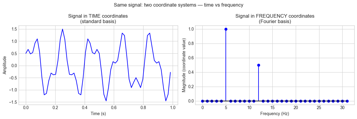
Dominant frequency coordinates:
  freq=5.0 Hz, magnitude=1.000
  freq=12.0 Hz, magnitude=0.500
  freq=25.0 Hz, magnitude=0.000
# --- Experiment 2: Orthonormal vs oblique — computational cost ---
# Hypothesis: Orthonormal coordinate extraction is O(n) (dot products).
# General basis requires solving a linear system: O(n^2) or O(n^3).

import numpy as np
import time

DIMS = [10, 100, 500, 1000, 2000]  # <-- try larger values

times_ortho = []
times_oblique = []
N_REPS = 20

rng = np.random.default_rng(0)

for n in DIMS:
    # Orthonormal basis via QR
    A = rng.standard_normal((n, n))
    Q, _ = np.linalg.qr(A)
    v = rng.standard_normal(n)

    # Time orthonormal extraction
    start = time.perf_counter()
    for _ in range(N_REPS):
        c = Q.T @ v  # just a matrix-vector product
    times_ortho.append((time.perf_counter() - start) / N_REPS * 1000)

    # Oblique basis (random independent vectors)
    B = rng.standard_normal((n, n))
    start = time.perf_counter()
    for _ in range(N_REPS):
        c = np.linalg.solve(B, v)  # requires O(n^2) to O(n^3)
    times_oblique.append((time.perf_counter() - start) / N_REPS * 1000)

import matplotlib.pyplot as plt
plt.style.use('seaborn-v0_8-whitegrid')

fig, ax = plt.subplots(figsize=(8, 4))
ax.loglog(DIMS, times_ortho, 'bo-', lw=2, markersize=7, label='Orthonormal (Bᵀv)')
ax.loglog(DIMS, times_oblique, 'rs-', lw=2, markersize=7, label='Oblique (solve Bc=v)')
ax.set_xlabel('Dimension n')
ax.set_ylabel('Time per extraction (ms)')
ax.set_title('Coordinate extraction cost:\northonormal vs oblique basis')
ax.legend()
plt.tight_layout()
plt.show()

print(f"{'n':>8}  {'ortho (ms)':>12}  {'oblique (ms)':>14}  {'speedup':>8}")
for n, to, tb in zip(DIMS, times_ortho, times_oblique):
    print(f"  {n:6d}  {to:12.4f}  {tb:14.4f}  {tb/to:8.1f}x")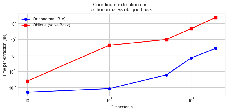
       n    ortho (ms)    oblique (ms)   speedup
      10        0.0049          0.0247       5.0x
     100        0.0082          4.2547     519.5x
     500        0.0596          9.6105     161.3x
    1000        0.6712         46.0874      68.7x
    2000        2.7254        229.2729      84.1x
7. Exercises
Easy 1. Vector v = (3, 4) in standard coordinates. Find its coordinates in the basis B = {(1, 1)/√2, (−1, 1)/√2}. Verify by reconstructing v from the computed coordinates.
Easy 2. If B is an orthonormal basis matrix (columns orthonormal), write a one-line expression for the coordinate vector of v in that basis. Why is this formula valid?
Medium 1. A robotics sensor gives position readings in a local frame with basis b₁ = (cos30°, sin30°), b₂ = (−sin30°, cos30°). The sensor reports a position of (2.0, 1.5) in its local frame. Find the position in world (standard) coordinates.
Medium 2. Two coordinate systems share the same origin. The first has basis {(1,0,0), (0,1,0), (0,0,1)} and the second has basis {(1,1,0)/√2, (−1,1,0)/√2, (0,0,1)}. Build the change-of-basis matrix from system 1 to system 2 and verify it is orthonormal (Rᵀ = R⁻¹).
Hard. Implement a 2D coordinate system visualizer: given any two linearly independent vectors as a basis, draw the resulting coordinate grid and allow the user to click a point on the plot and read off its coordinates in that basis. (Use matplotlib’s interactive mode or parametric line plotting.)
8. Mini Project
# --- Mini Project: Multi-Frame Robot Position Tracker ---
#
# Problem: A robot has a body frame, a camera frame, and a world frame.
# All three are coordinate systems. Sensor data arrives in the camera frame;
# plans are made in the world frame. Build a transformation pipeline.

import numpy as np
import matplotlib.pyplot as plt

plt.style.use('seaborn-v0_8-whitegrid')
rng = np.random.default_rng(0)

# --- Frame definitions ---
# World frame: standard (identity)
# Body frame: robot is at position (3, 2) in world, rotated 30° CCW
ROBOT_POS_WORLD = np.array([3.0, 2.0])
ROBOT_ANGLE_DEG = 30.0   # <-- try different angles
theta = np.radians(ROBOT_ANGLE_DEG)

# Body frame basis vectors (in world coordinates)
body_x = np.array([np.cos(theta), np.sin(theta)])   # robot's forward direction
body_y = np.array([-np.sin(theta), np.cos(theta)])  # robot's left direction
B_body = np.column_stack([body_x, body_y])

# Camera frame: mounted on robot, offset (0.5, 0) in body frame, rotated 15° CCW
CAM_OFFSET_BODY = np.array([0.5, 0.0])
CAM_ANGLE_DEG = 15.0     # <-- try different camera angles
phi = np.radians(CAM_ANGLE_DEG)
cam_x_body = np.array([np.cos(phi), np.sin(phi)])
cam_y_body = np.array([-np.sin(phi), np.cos(phi)])
B_cam_in_body = np.column_stack([cam_x_body, cam_y_body])

# --- Transformation pipeline ---
def camera_to_body(p_cam):
    """Convert camera-frame coordinates to body-frame coordinates."""
    return B_cam_in_body @ p_cam + CAM_OFFSET_BODY

def body_to_world(p_body):
    """Convert body-frame coordinates to world-frame coordinates."""
    return B_body @ p_body + ROBOT_POS_WORLD

def camera_to_world(p_cam):
    """Full pipeline: camera -> body -> world."""
    return body_to_world(camera_to_body(p_cam))

# --- Simulate obstacle detections in camera frame ---
obstacles_cam = [
    np.array([2.0, 0.3]),
    np.array([1.5, -0.5]),
    np.array([3.0, 0.0]),
]

print("Obstacle positions in different frames:")
print(f"{'Camera frame':>20}  {'Body frame':>20}  {'World frame':>20}")
obstacles_world = []
for obs_cam in obstacles_cam:
    obs_body = camera_to_body(obs_cam)
    obs_world = body_to_world(obs_body)
    obstacles_world.append(obs_world)
    print(f"  ({obs_cam[0]:5.2f},{obs_cam[1]:5.2f})    "
          f"  ({obs_body[0]:5.2f},{obs_body[1]:5.2f})    "
          f"  ({obs_world[0]:5.2f},{obs_world[1]:5.2f})")

# --- Visualization ---
fig, ax = plt.subplots(figsize=(8, 8))

# World frame grid
for i in np.arange(-1, 7):
    ax.axhline(i, color='lightblue', lw=0.7, alpha=0.5)
    ax.axvline(i, color='lightblue', lw=0.7, alpha=0.5)

# Robot body frame
ax.quiver(*ROBOT_POS_WORLD, *body_x, color='blue', scale=4,
          width=0.005, label='Robot body frame')
ax.quiver(*ROBOT_POS_WORLD, *body_y, color='blue', scale=4, width=0.005)

# Camera position in world
cam_pos_world = body_to_world(CAM_OFFSET_BODY)
cam_x_world = B_body @ cam_x_body
cam_y_world = B_body @ cam_y_body
ax.quiver(*cam_pos_world, *cam_x_world, color='green', scale=5,
          width=0.005, label='Camera frame')
ax.quiver(*cam_pos_world, *cam_y_world, color='green', scale=5, width=0.005)

# Robot and camera markers
ax.plot(*ROBOT_POS_WORLD, 'bs', markersize=12, zorder=5, label='Robot origin')
ax.plot(*cam_pos_world, 'g^', markersize=10, zorder=5, label='Camera')

# Obstacles in world frame
for i, (obs_cam, obs_world) in enumerate(zip(obstacles_cam, obstacles_world)):
    ax.plot(*obs_world, 'ro', markersize=10, zorder=5)
    ax.text(obs_world[0]+0.1, obs_world[1]+0.1,
            f'obs{i} cam=({obs_cam[0]:.1f},{obs_cam[1]:.1f})\n'
            f'world=({obs_world[0]:.2f},{obs_world[1]:.2f})',
            fontsize=8)

ax.set_xlim(-1, 7); ax.set_ylim(-1, 7)
ax.set_xlabel('World x'); ax.set_ylabel('World y')
ax.set_title(f'Robot at ({ROBOT_POS_WORLD[0]},{ROBOT_POS_WORLD[1]}), '
              f'rotated {ROBOT_ANGLE_DEG}°\nCamera offset, rotated {CAM_ANGLE_DEG}°')
ax.legend(loc='upper left')
ax.set_aspect('equal')
plt.tight_layout()
plt.show()
9. Chapter Summary & Connections
What was covered:
A coordinate system = a basis. Coordinates are the unique representation of a vector in that basis.
Orthonormal bases give the simplest coordinate extraction: cᵢ = bᵢ · v (dot product only).
The change-of-basis matrix P converts coordinates from one system to another: [v]_B2 = P[v]_B1.
Coordinate systems are fundamental to signal processing (Fourier), graphics (frame transforms), and ML (feature spaces).
Backward connection: This chapter applies ch139 (Basis) and ch141 (Independence) concretely: a coordinate system exists because a basis is independent (unique coordinates) and spans the space (every vector is reachable). (Introduced in ch139, ch141.)
Forward connections:
In ch143 (Vector Transformations), we examine what happens to coordinate systems when a linear map is applied — transformations act on both the vectors and their coordinate representations.
This will reappear in ch183 (Eigenvalue Computation): the eigenvector basis is the coordinate system in which a matrix acts as a pure scaling — the simplest possible representation.
In ch186 (PCA), principal components define a new coordinate system that maximally decorrelates the data — coordinate change as a tool for insight.