Prerequisites: ch140 (Span), ch139 (Basis and Dimension), ch127 (Linear Combination), ch128 (Vector Length/Norm)
You will learn:
The formal definition of linear independence and why it matters
How to test a set of vectors for independence computationally
The geometric interpretation: no vector is “trapped” in the span of the others
How independence relates to the determinant and rank
Why independence is the key condition in basis, solution uniqueness, and model identifiability
Environment: Python 3.x, numpy, matplotlib
1. Concept¶
A set of vectors {v₁, v₂, ..., vₖ} is linearly independent if the only solution to
c₁v₁ + c₂v₂ + ... + cₖvₖ = 0is the trivial one: c₁ = c₂ = ... = cₖ = 0.
If a non-trivial solution exists (at least one cᵢ ≠ 0), the set is linearly dependent — meaning at least one vector can be written as a linear combination of the others.
Why it matters:
A basis requires independence. Without it, coordinates are not unique.
In a linear system Ax = b, independence of columns guarantees a unique solution when one exists.
In ML, independent features carry non-redundant information. Dependent features cause identifiability problems (multicollinearity).
Common misconceptions:
“Orthogonal vectors are always independent, but independent vectors aren’t always orthogonal.” Both parts are true — independence is a weaker condition than orthogonality.
“If all vectors in a set are non-zero, they are independent.” False — (1,0) and (2,0) are both non-zero but linearly dependent.
“Linear independence depends on the magnitude of vectors.” False — it depends only on direction. Scaling a vector does not affect independence of the set.
2. Intuition & Mental Models¶
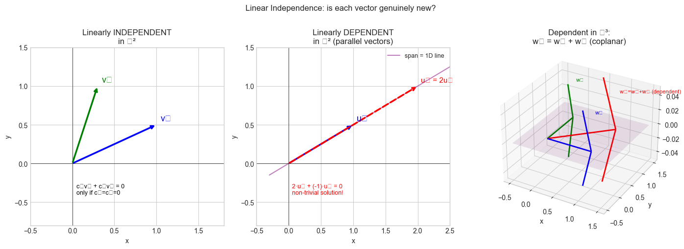
Geometric model: A set of vectors is linearly independent if no vector in the set lies in the span of the others. Each vector points in a direction that the others cannot collectively reach.
In ℝ²: two vectors are independent iff they are not parallel (not one a multiple of the other).
In ℝ³: three vectors are independent iff none lies in the plane spanned by the other two.
Dependence means you have a “shortcut” — you can express one vector using the others, so it contributes nothing new to the span. Independence means every vector is genuinely novel.
Computational model: Think of independence as a uniqueness condition. Given a set of vectors, you build a matrix A with those vectors as columns. The homogeneous system Ac = 0 has only the trivial solution c = 0 iff the columns are independent. This is equivalent to A having full column rank — all singular values are non-zero.
Recall from ch140 (Span): adding a dependent vector does not change the span. Independence is precisely the condition that says every vector in your set does change the span — each one adds a new dimension.
3. Visualization¶
# --- Visualization: Independent vs dependent vectors in R^2 and R^3 ---

import numpy as np
import matplotlib.pyplot as plt
from mpl_toolkits.mplot3d import Axes3D

plt.style.use('seaborn-v0_8-whitegrid')
fig = plt.figure(figsize=(14, 5))

# --- Panel 1: Independent in R^2 ---
ax1 = fig.add_subplot(131)
v1 = np.array([1.0, 0.5])
v2 = np.array([0.3, 1.0])  # not parallel to v1

ax1.annotate('', xy=v1, xytext=[0,0], arrowprops=dict(arrowstyle='->', color='blue', lw=2.5))
ax1.annotate('', xy=v2, xytext=[0,0], arrowprops=dict(arrowstyle='->', color='green', lw=2.5))
ax1.text(v1[0]+0.05, v1[1]+0.05, 'v₁', fontsize=13, color='blue')
ax1.text(v2[0]+0.05, v2[1]+0.05, 'v₂', fontsize=13, color='green')
# Show that 0*v1 + 0*v2 = 0 is the only solution
ax1.text(0.05, -0.4, 'c₁v₁ + c₂v₂ = 0\nonly if c₁=c₂=0', fontsize=9, color='black')
ax1.set_xlim(-0.5, 1.8); ax1.set_ylim(-0.8, 1.5)
ax1.set_title('Linearly INDEPENDENT\nin ℝ²')
ax1.axhline(0, color='k', lw=0.5); ax1.axvline(0, color='k', lw=0.5)
ax1.set_xlabel('x'); ax1.set_ylabel('y')

# --- Panel 2: Dependent in R^2 ---
ax2 = fig.add_subplot(132)
u1 = np.array([1.0, 0.5])
u2 = np.array([2.0, 1.0])  # = 2 * u1

ax2.annotate('', xy=u1, xytext=[0,0], arrowprops=dict(arrowstyle='->', color='blue', lw=2.5))
ax2.annotate('', xy=u2, xytext=[0,0], arrowprops=dict(arrowstyle='->', color='red', lw=2.5, linestyle='dashed'))
ax2.text(u1[0]+0.05, u1[1]+0.05, 'u₁', fontsize=13, color='blue')
ax2.text(u2[0]+0.05, u2[1]+0.05, 'u₂ = 2u₁', fontsize=11, color='red')
t = np.linspace(-0.3, 2.5, 100)
ax2.plot(t, 0.5*t, 'purple', lw=1.5, alpha=0.5, label='span = 1D line')
ax2.text(0.05, -0.4, '2·u₁ + (-1)·u₂ = 0\nnon-trivial solution!', fontsize=9, color='red')
ax2.set_xlim(-0.5, 2.5); ax2.set_ylim(-0.8, 1.5)
ax2.set_title('Linearly DEPENDENT\nin ℝ² (parallel vectors)')
ax2.legend(fontsize=9)
ax2.axhline(0, color='k', lw=0.5); ax2.axvline(0, color='k', lw=0.5)
ax2.set_xlabel('x'); ax2.set_ylabel('y')

# --- Panel 3: Three vectors in R^3 — dependent (coplanar) ---
ax3 = fig.add_subplot(133, projection='3d')
w1 = np.array([1., 0., 0.])
w2 = np.array([0., 1., 0.])
w3 = np.array([1., 1., 0.])  # = w1 + w2 — dependent!

colors = ['blue', 'green', 'red']
labels = ['w₁', 'w₂', 'w₃=w₁+w₂ (dependent)']
for w, c, l in zip([w1, w2, w3], colors, labels):
    ax3.quiver(0, 0, 0, *w, color=c, lw=2, arrow_length_ratio=0.2)
    ax3.text(*(w + 0.05), l, fontsize=8, color=c)

s_vals = np.linspace(-0.5, 1.5, 10)
t_vals = np.linspace(-0.5, 1.5, 10)
S, T = np.meshgrid(s_vals, t_vals)
ax3.plot_surface(S, T, np.zeros_like(S), alpha=0.1, color='purple')
ax3.set_title('Dependent in ℝ³:\nw₃ = w₁ + w₂ (coplanar)')
ax3.set_xlabel('x'); ax3.set_ylabel('y'); ax3.set_zlabel('z')

plt.suptitle('Linear Independence: is each vector genuinely new?', fontsize=12, y=1.01)
plt.tight_layout()
plt.show()
C:\Users\user\AppData\Local\Temp\ipykernel_256\114513997.py:64: UserWarning: Glyph 8477 (\N{DOUBLE-STRUCK CAPITAL R}) missing from font(s) Arial.
plt.tight_layout()
C:\Users\user\AppData\Local\Temp\ipykernel_256\114513997.py:64: UserWarning: Glyph 8321 (\N{SUBSCRIPT ONE}) missing from font(s) Arial.
plt.tight_layout()
C:\Users\user\AppData\Local\Temp\ipykernel_256\114513997.py:64: UserWarning: Glyph 8322 (\N{SUBSCRIPT TWO}) missing from font(s) Arial.
plt.tight_layout()
C:\Users\user\AppData\Local\Temp\ipykernel_256\114513997.py:64: UserWarning: Glyph 8323 (\N{SUBSCRIPT THREE}) missing from font(s) Arial.
plt.tight_layout()
c:\Users\user\OneDrive\Documents\book\.venv\Lib\site-packages\IPython\core\pylabtools.py:170: UserWarning: Glyph 8321 (\N{SUBSCRIPT ONE}) missing from font(s) Arial.
fig.canvas.print_figure(bytes_io, **kw)
c:\Users\user\OneDrive\Documents\book\.venv\Lib\site-packages\IPython\core\pylabtools.py:170: UserWarning: Glyph 8322 (\N{SUBSCRIPT TWO}) missing from font(s) Arial.
fig.canvas.print_figure(bytes_io, **kw)
c:\Users\user\OneDrive\Documents\book\.venv\Lib\site-packages\IPython\core\pylabtools.py:170: UserWarning: Glyph 8323 (\N{SUBSCRIPT THREE}) missing from font(s) Arial.
fig.canvas.print_figure(bytes_io, **kw)
c:\Users\user\OneDrive\Documents\book\.venv\Lib\site-packages\IPython\core\pylabtools.py:170: UserWarning: Glyph 8477 (\N{DOUBLE-STRUCK CAPITAL R}) missing from font(s) Arial.
fig.canvas.print_figure(bytes_io, **kw)
4. Mathematical Formulation¶
Definition:
{v₁, ..., vₖ} is linearly independent iff:
c₁v₁ + c₂v₂ + ... + cₖvₖ = 0 ⟹ c₁ = c₂ = ... = cₖ = 0Equivalently (matrix form): Let A = [v₁ | ... | vₖ]. Then:
columns of A are linearly independent
  ⟺  N(A) = {0}  (null space is trivial)
  ⟺  rank(A) = k  (full column rank)
  ⟺  A†A is invertible  (Gram matrix is non-singular)
  ⟺  all singular values of A are non-zero
For square matrices: n vectors in ℝⁿ are independent iff their matrix has non-zero determinant:
det([v₁ | ... | vₙ]) ≠ 0 ⟺ {v₁, ..., vₙ} linearly independent(Determinants are formalized in ch158.)
Dependence relation: If {v₁, ..., vₖ} is dependent, some vector can be expressed in terms of the others. Specifically, if the solution to Ac = 0 gives cⱼ ≠ 0, then:
vⱼ = - (1/cⱼ) Σᵢ≠ⱼ cᵢ vᵢMaximum independent set: In ℝⁿ, any set of more than n vectors is linearly dependent — you cannot have more than n independent directions. (This is the Steinitz exchange lemma used in ch139.)
5. Python Implementation¶
# --- Implementation: Independence testing ---

import numpy as np


def are_independent(vectors, tol=1e-10):
    """
    Test whether a set of vectors is linearly independent.

    Uses rank: columns are independent iff rank equals number of vectors.

    Args:
        vectors: list of np.ndarray, each shape (n,)
        tol: float — threshold for singular value to be 'non-zero'

    Returns:
        dict with 'independent' (bool), 'rank', 'n_vectors', 'min_singular_value'
    """
    A = np.column_stack(vectors)
    s = np.linalg.svd(A, compute_uv=False)
    rank = np.sum(s > tol)
    n = len(vectors)
    return {
        'independent': rank == n,
        'rank': rank,
        'n_vectors': n,
        'min_singular_value': float(s.min())
    }


def find_dependence_relation(vectors, tol=1e-10):
    """
    If vectors are dependent, find the non-trivial combination that equals zero.

    Returns:
        np.ndarray of coefficients c such that sum(cᵢ * vᵢ) ≈ 0,
        or None if independent.
    """
    A = np.column_stack(vectors)
    U, s, Vt = np.linalg.svd(A, full_matrices=True)
    # The right singular vector for the smallest singular value
    # is the 'most null' direction
    if s.min() > tol:
        return None  # independent
    # The last row of Vt corresponds to smallest singular value
    c = Vt[-1]
    return c


# --- Tests ---
print("=== Independence tests ===")

cases = [
    ([np.array([1.,0.]), np.array([0.,1.])], "standard basis R^2"),
    ([np.array([1.,2.]), np.array([2.,4.])], "parallel vectors (dependent)"),
    ([np.array([1.,1.,0.]), np.array([0.,1.,1.]), np.array([1.,0.,1.])], "3 in R^3 (indep?)"),
    ([np.array([1.,2.,3.]), np.array([2.,4.,6.]), np.array([0.,1.,0.])], "one is multiple"),
]

for vecs, name in cases:
    result = are_independent(vecs)
    print(f"\n{name}:")
    print(f"  Independent: {result['independent']}")
    print(f"  Rank={result['rank']}, n={result['n_vectors']}, min_sv={result['min_singular_value']:.2e}")
    if not result['independent']:
        c = find_dependence_relation(vecs)
        print(f"  Dependence relation: {c.round(4)}")
        print(f"  Verify: {sum(ci*vi for ci,vi in zip(c,vecs)).round(10)}")
=== Independence tests ===
standard basis R^2:
Independent: True
Rank=2, n=2, min_sv=1.00e+00
parallel vectors (dependent):
Independent: False
Rank=1, n=2, min_sv=1.99e-16
Dependence relation: [-0.8944 0.4472]
Verify: [0. 0.]
3 in R^3 (indep?):
Independent: True
Rank=3, n=3, min_sv=1.00e+00
one is multiple:
Independent: False
Rank=2, n=3, min_sv=8.86e-16
Dependence relation: [ 0.8944 -0.4472 -0. ]
Verify: [-0. -0. -0.]
# --- Gram matrix test for independence ---
# The Gram matrix G = A^T A is positive definite iff columns of A are independent

import numpy as np


def gram_matrix_test(vectors, tol=1e-10):
    """
    Gram matrix G = A^T @ A.
    G is positive definite (all eigenvalues > 0) iff vectors are independent.

    Args:
        vectors: list of np.ndarray

    Returns:
        dict with 'G' (matrix), 'eigenvalues', 'is_pos_def', 'independent'
    """
    A = np.column_stack(vectors)
    G = A.T @ A   # Gram matrix: G[i,j] = vi . vj (dot products)
    eigvals = np.linalg.eigvalsh(G)
    is_pos_def = bool(eigvals.min() > tol)
    return {
        'G': G,
        'eigenvalues': eigvals,
        'is_pos_def': is_pos_def,
        'independent': is_pos_def
    }


# Independent vectors
vecs_ind = [np.array([1.,0.,0.]), np.array([0.,1.,0.])]
r_ind = gram_matrix_test(vecs_ind)
print("Independent vectors:")
print(f"  Gram matrix:\n{r_ind['G']}")
print(f"  Eigenvalues: {r_ind['eigenvalues'].round(6)}")
print(f"  Positive definite: {r_ind['is_pos_def']}")
print()

# Dependent vectors
vecs_dep = [np.array([1.,2.,0.]), np.array([2.,4.,0.])]
r_dep = gram_matrix_test(vecs_dep)
print("Dependent vectors:")
print(f"  Gram matrix:\n{r_dep['G']}")
print(f"  Eigenvalues: {r_dep['eigenvalues'].round(6)}")
print(f"  Positive definite: {r_dep['is_pos_def']}")
print("  (Note: zero eigenvalue = singular Gram matrix = dependent columns)")
Independent vectors:
Gram matrix:
[[1. 0.]
[0. 1.]]
Eigenvalues: [1. 1.]
Positive definite: True
Dependent vectors:
Gram matrix:
[[ 5. 10.]
[10. 20.]]
Eigenvalues: [ 0. 25.]
Positive definite: False
(Note: zero eigenvalue = singular Gram matrix = dependent columns)
6. Experiments¶
# --- Experiment 1: Near-independence and numerical conditioning ---
# Hypothesis: Vectors that are "almost" parallel are technically independent
# but numerically problematic. The minimum singular value measures this.

import numpy as np
import matplotlib.pyplot as plt

plt.style.use('seaborn-v0_8-whitegrid')

# Two vectors at angle theta to each other
ANGLES_DEG = [90, 60, 30, 10, 5, 1, 0.1]  # <-- modify this list

min_svs = []
for deg in ANGLES_DEG:
    theta = np.radians(deg)
    v1 = np.array([1.0, 0.0])
    v2 = np.array([np.cos(theta), np.sin(theta)])
    A = np.column_stack([v1, v2])
    s = np.linalg.svd(A, compute_uv=False)
    min_svs.append(s.min())

fig, ax = plt.subplots(figsize=(8, 4))
ax.semilogy(ANGLES_DEG, min_svs, 'bo-', markersize=8, linewidth=2)
ax.axhline(1e-10, color='red', linestyle='--', label='Numerical zero threshold')
ax.set_xlabel('Angle between vectors (degrees)')
ax.set_ylabel('Minimum singular value (log scale)')
ax.set_title('Near-independence: min singular value → 0 as vectors become parallel')
ax.legend()
plt.tight_layout()
plt.show()

print(f"{'Angle':>10}  {'Min SV':>15}  {'Numerically indep':>18}")
for deg, sv in zip(ANGLES_DEG, min_svs):
    print(f"  {deg:8.1f}°  {sv:15.2e}  {sv > 1e-10!s:>18}")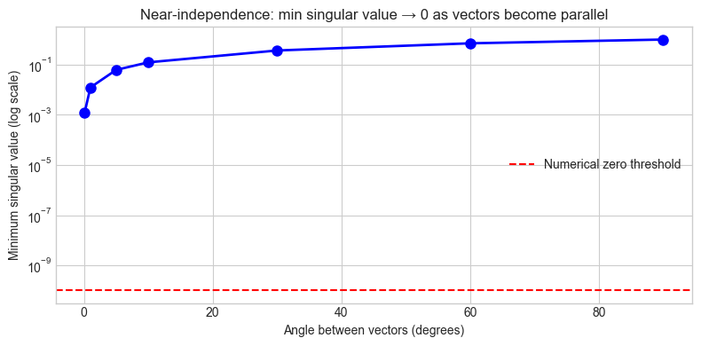
     Angle           Min SV   Numerically indep
      90.0°         1.00e+00                True
      60.0°         7.07e-01                True
      30.0°         3.66e-01                True
      10.0°         1.23e-01                True
       5.0°         6.17e-02                True
       1.0°         1.23e-02                True
       0.1°         1.23e-03                True
# --- Experiment 2: Random vectors in high dimensions ---
# Hypothesis: Random vectors in high dimensions are almost always independent.
# The probability of dependence is zero for continuous distributions.

import numpy as np

rng = np.random.default_rng(0)

N_TRIALS = 200  # <-- modify
DIM = 10        # <-- try 2, 5, 100
K = 5           # number of vectors (must be <= DIM to have hope of independence)

independent_count = 0
min_svs = []

for _ in range(N_TRIALS):
    A = rng.standard_normal((DIM, K))
    s = np.linalg.svd(A, compute_uv=False)
    min_svs.append(s.min())
    if s.min() > 1e-10:
        independent_count += 1

print(f"In {N_TRIALS} trials with {K} random vectors in R^{DIM}:")
print(f"  Independent: {independent_count}/{N_TRIALS} = {100*independent_count/N_TRIALS:.1f}%")
print(f"  Min singular value — mean: {np.mean(min_svs):.4f}, min: {np.min(min_svs):.4f}")
print()
if K > DIM:
    print(f"Note: k={K} > n={DIM}, so vectors must be dependent by dimension argument.")
In 200 trials with 5 random vectors in R^10:
Independent: 200/200 = 100.0%
Min singular value — mean: 1.3341, min: 0.5266
# --- Experiment 3: Multicollinearity in data — a practical consequence ---
# Hypothesis: Dependent features in a dataset make the coefficient solution
# unstable (many solutions, huge coefficients).

import numpy as np

rng = np.random.default_rng(42)
N = 50

x1 = rng.standard_normal(N)
x2 = x1 + rng.normal(0, NOISE, N)  if (NOISE := 0.01) else x1  # nearly = x1
# <-- try NOISE = 1.0 (independent), 0.01 (nearly dep), 0.0 (exactly dep)
NOISE = 0.01
x2 = x1 + rng.normal(0, NOISE, N)

y = 2*x1 + 3*x2 + rng.normal(0, 0.1, N)  # true coefficients: 2, 3

X = np.column_stack([x1, x2])
coeffs = np.linalg.lstsq(X, y, rcond=None)[0]
condition_number = np.linalg.cond(X)

print(f"Noise level on x2: {NOISE}")
print(f"Correlation(x1,x2): {np.corrcoef(x1,x2)[0,1]:.6f}")
print(f"Condition number of X: {condition_number:.2e}")
print(f"Fitted coefficients: [{coeffs[0]:.4f}, {coeffs[1]:.4f}]")
print(f"True coefficients:   [2.0000, 3.0000]")
print()
print("As NOISE -> 0: x1 and x2 become dependent, condition number -> inf,")
print("and coefficients blow up even though their sum stays near 5.")
Noise level on x2: 0.01
Correlation(x1,x2): 0.999915
Condition number of X: 1.54e+02
Fitted coefficients: [2.0312, 2.9916]
True coefficients: [2.0000, 3.0000]
As NOISE -> 0: x1 and x2 become dependent, condition number -> inf,
and coefficients blow up even though their sum stays near 5.
7. Exercises¶
Easy 1. Determine by inspection (no code) whether each set is independent:
(a) {(1,0), (0,1), (1,1)} in ℝ²
(b) {(1,2,3), (0,0,0), (4,5,6)}
(c) {(1,0,0), (0,1,0)} in ℝ³
(Expected: a — dependent (3 vectors in 2D); b — dependent (zero vector); c — independent)
Easy 2. Write code that generates a random 4×3 matrix, checks if its columns are independent, and if not, finds and prints the dependence relation.
Medium 1. Given v₁ = (1, -1, 0), v₂ = (0, 1, -1), v₃ = (1, 0, -1): are these independent? If not, express one as a combination of the others using the dependence relation you find computationally.
Medium 2. The Gram-Schmidt process (introduced in ch135 — Orthogonality) converts an independent set into an orthonormal one. Write code that: (a) takes a list of independent vectors, (b) runs Gram-Schmidt, (c) verifies the result is orthonormal. What happens if the input vectors are dependent?
Hard. Condition number and independence: Write an experiment that generates pairs of unit vectors at angles θ ∈ [1°, 90°] and for each pair: (a) computes the condition number of the 2×2 matrix they form, (b) solves a linear system Ax = b and measures error magnitude. Plot how error scales with condition number. This demonstrates why near-dependence (multicollinearity) is a practical problem, not just a theoretical one.
8. Mini Project¶
# --- Mini Project: Feature Independence Auditor ---
#
# Problem: Before training a linear model, it is important to detect
# linearly dependent or near-dependent features. Dependent features
# cause infinite or unstable coefficient estimates.
#
# Build an auditor that:
# 1. Checks for exact and near-linear dependence
# 2. Identifies which features are redundant
# 3. Recommends a minimal independent feature set

import numpy as np
import matplotlib.pyplot as plt

plt.style.use('seaborn-v0_8-whitegrid')
rng = np.random.default_rng(0)

# --- Synthetic dataset with intentional redundancy ---
N, D = 100, 6
# True independent features
F_true = rng.standard_normal((N, 3))
# Derived features (linear combinations + noise)
F_derived = np.column_stack([
    2*F_true[:, 0] - F_true[:, 1] + rng.normal(0, 0.01, N),  # nearly = 2F0 - F1
    F_true[:, 2] + rng.normal(0, 0.01, N),                    # nearly = F2
    rng.standard_normal(N),                                    # truly independent noise
])
X = np.column_stack([F_true, F_derived])
feature_names = [f'F{i}' for i in range(D)]

print(f"Feature matrix X: {X.shape}")
print(f"Features: {feature_names}")
print()

# --- TODO 1: Compute singular values and identify near-zero ones ---
_, svs, Vt = np.linalg.svd(X, full_matrices=False)
print("Singular values of X:")
for i, sv in enumerate(svs):
    flag = " <-- near zero (dependent)" if sv < 1.0 else ""
    print(f"  σ{i+1} = {sv:.4f}{flag}")

# --- TODO 2: Find independent feature subset via QR with pivoting ---
# We use SVD-based selection: keep top-k features where k = rank
rank = np.sum(svs > 1.0)  # threshold — tune based on problem
print(f"\nEffective rank: {rank}  (independent dimensions)")

# The rows of Vt corresponding to top singular values identify the important directions
# Simpler: use greedy column selection
def select_independent_columns(X, tol=1.0):
    """
    Greedily select columns of X to form an independent set.
    Returns indices of selected columns.
    """
    selected = []
    for i in range(X.shape[1]):
        candidate = selected + [i]
        if np.linalg.matrix_rank(X[:, candidate], tol=tol) > len(selected):
            selected.append(i)
    return selected

selected_idx = select_independent_columns(X)
print(f"Selected independent features: {[feature_names[i] for i in selected_idx]}")
print(f"  (indices: {selected_idx})")

# --- Visualization: singular value spectrum ---
fig, (ax1, ax2) = plt.subplots(1, 2, figsize=(12, 4))

ax1.bar(range(1, len(svs)+1), svs, color=['green' if sv > 1.0 else 'red' for sv in svs])
ax1.axhline(1.0, color='orange', linestyle='--', label='Independence threshold')
ax1.set_xlabel('Singular value index')
ax1.set_ylabel('Singular value')
ax1.set_title('Singular value spectrum\nGreen = independent, Red = redundant')
ax1.legend()

# Condition numbers for original vs reduced feature set
X_reduced = X[:, selected_idx]
cond_orig = np.linalg.cond(X)
cond_red = np.linalg.cond(X_reduced)
ax2.bar(['Original (6 features)', f'Reduced ({len(selected_idx)} features)'],
        [cond_orig, cond_red], color=['red', 'green'])
ax2.set_ylabel('Condition number (log scale)')
ax2.set_yscale('log')
ax2.set_title('Condition number before/after\nremoving dependent features')

plt.tight_layout()
plt.show()

print(f"\nCondition number: original={cond_orig:.2e}, reduced={cond_red:.2e}")
9. Chapter Summary & Connections¶
What was covered:
Linear independence: the only way to combine the vectors to get zero is the trivial way.
Independence ⟺ full column rank ⟺ trivial null space ⟺ positive definite Gram matrix.
The minimum singular value measures how close a set is to being dependent — it is the key numerical indicator.
More than n vectors in ℝⁿ must be dependent.
Near-independence (multicollinearity) causes numerically unstable computations.
Backward connection: This completes the trio from ch138–140: subspaces (ch138), span (ch140), and now independence. A basis = independent + spans the space. Dimension = size of any basis. The three concepts are inseparable.
Forward connections:
In ch142 (Coordinate Systems), independent vectors form the axes of a coordinate system — uniqueness of coordinates follows from independence.
This will reappear in ch160 (Systems of Linear Equations): full column rank (independent columns) guarantees at most one solution; full row rank (independent rows) guarantees at least one.
In ch176 (Eigenvectors), eigenspaces from distinct eigenvalues are linearly independent — a critical fact for diagonalization in ch177.
In Part IX (ch271–300), multicollinearity detection and VIF (variance inflation factor) are the applied statistics version of this chapter’s numerical experiments.