Prerequisites: ch125 (Vector Addition), ch126 (Scalar Multiplication), ch128 (Norm), ch130 (Direction Vectors), ch133 (Angles Between Vectors)
You will learn:
How physical quantities — force, velocity, acceleration — are vectors
Newton’s second law and superposition as vector operations
Work, power, and torque via dot and cross products
How to simulate basic Newtonian mechanics with vectors in code
Why physical intuition about vectors transfers directly to data science
Environment: Python 3.x, numpy, matplotlib
1. Concept
Physics was the original motivation for vectors. Quantities like force, velocity, and acceleration cannot be fully described by a single number — they have both magnitude and direction. Vectors provide the natural language.
Scalar vs vector quantities:
Scalars: mass (kg), temperature (°C), speed (m/s), energy (J) — magnitude only
Vectors: force (N), velocity (m/s with direction), acceleration (m/s²), displacement (m), torque (N·m)
Why this chapter matters beyond physics: The structures here — superposition, work as a dot product, torque as a cross product — are templates that reappear throughout data science and ML. Gradient descent is an application of force-like vectors. Attention mechanisms compute scaled dot products. The physics intuition makes the math visceral.
Common misconception: “Physics vectors are different from math vectors.” They are the same object. A force vector F ∈ ℝ³ satisfies all eight axioms from ch137. The physics gives intuition; the math gives precision.
2. Intuition & Mental Models
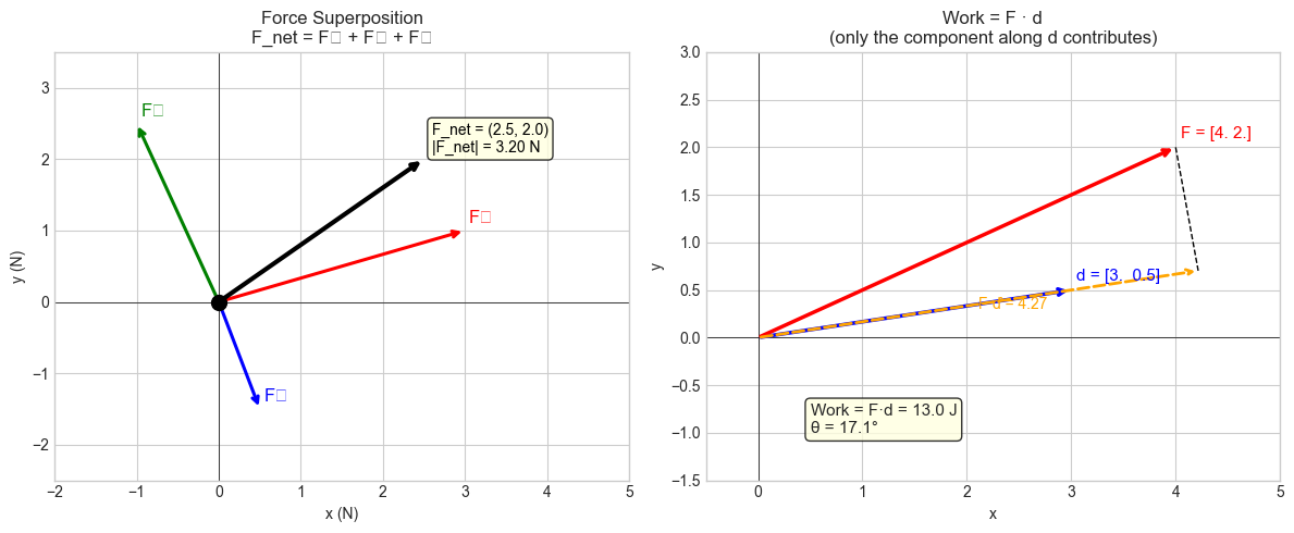
Superposition = vector addition: Multiple forces acting on an object combine by vector addition. The net force is the vector sum. This is why vector addition (introduced in ch125) has the tip-to-tail interpretation — it models what forces physically do.
Work = dot product: When you push an object with force F through displacement d, only the component of force along the direction of motion does useful work. Work = F · d = ‖F‖‖d‖cos θ. (The projection formula from ch134 makes this concrete: work is the projection of force onto displacement, scaled by displacement magnitude.)
Torque = cross product: The rotational effect of a force depends on both the force magnitude and how far from the pivot it acts. Torque τ = r × F is a cross product (introduced in ch136) — its magnitude is the “turning power,” its direction gives the axis of rotation.
Computational model: In a physics simulation, every object has state vectors: position x ∈ ℝ³, velocity v ∈ ℝ³, acceleration a ∈ ℝ³. Each timestep: v ← v + a·Δt, x ← x + v·Δt. This is Euler integration — a purely vector operation.
3. Visualization
# --- Visualization: Force superposition and work ---

import numpy as np
import matplotlib.pyplot as plt

plt.style.use('seaborn-v0_8-whitegrid')
fig, axes = plt.subplots(1, 2, figsize=(12, 5))

# --- Panel 1: Force superposition ---
ax = axes[0]
F1 = np.array([3.0, 1.0])   # Force 1
F2 = np.array([-1.0, 2.5])  # Force 2
F3 = np.array([0.5, -1.5])  # Force 3
F_net = F1 + F2 + F3

origin = np.array([0., 0.])
forces = [(F1,'red','F₁'), (F2,'green','F₂'), (F3,'blue','F₃')]
for F, c, label in forces:
    ax.annotate('', xy=F, xytext=origin,
                arrowprops=dict(arrowstyle='->', color=c, lw=2.2))
    ax.text(F[0]+0.05, F[1]+0.1, label, fontsize=12, color=c)

ax.annotate('', xy=F_net, xytext=origin,
            arrowprops=dict(arrowstyle='->', color='black', lw=3))
ax.text(F_net[0]+0.1, F_net[1]+0.1,
        f'F_net = ({F_net[0]:.1f}, {F_net[1]:.1f})\n|F_net| = {np.linalg.norm(F_net):.2f} N',
        fontsize=10, color='black',
        bbox=dict(boxstyle='round', facecolor='lightyellow', alpha=0.8))
ax.plot(0, 0, 'ko', markersize=10, zorder=5)
ax.set_xlim(-2, 5); ax.set_ylim(-2.5, 3.5)
ax.set_xlabel('x (N)'); ax.set_ylabel('y (N)')
ax.set_title('Force Superposition\nF_net = F₁ + F₂ + F₃')
ax.axhline(0, color='k', lw=0.5); ax.axvline(0, color='k', lw=0.5)

# --- Panel 2: Work = dot product ---
ax2 = axes[1]
F = np.array([4.0, 2.0])   # force vector
d = np.array([3.0, 0.5])   # displacement vector

work = F @ d
theta = np.degrees(np.arccos(F@d / (np.linalg.norm(F)*np.linalg.norm(d))))

# Project F onto d
d_unit = d / np.linalg.norm(d)
F_proj = (F @ d_unit) * d_unit
F_perp = F - F_proj

ax2.annotate('', xy=d, xytext=origin, arrowprops=dict(arrowstyle='->', color='blue', lw=2.5))
ax2.annotate('', xy=F, xytext=origin, arrowprops=dict(arrowstyle='->', color='red', lw=2.5))
ax2.annotate('', xy=F_proj, xytext=origin,
             arrowprops=dict(arrowstyle='->', color='orange', lw=2, linestyle='dashed'))
ax2.plot([F[0], F_proj[0]], [F[1], F_proj[1]], 'k--', lw=1)

ax2.text(d[0]+0.05, d[1]+0.1, f'd = {d}', fontsize=11, color='blue')
ax2.text(F[0]+0.05, F[1]+0.1, f'F = {F}', fontsize=11, color='red')
ax2.text(F_proj[0]/2, F_proj[1]-0.4, f'F·d̂ = {np.linalg.norm(F_proj):.2f}', fontsize=10, color='orange')
ax2.text(0.5, -1.0,
         f'Work = F·d = {work:.1f} J\nθ = {theta:.1f}°',
         fontsize=11, bbox=dict(boxstyle='round', facecolor='lightyellow', alpha=0.8))
ax2.set_xlim(-0.5, 5); ax2.set_ylim(-1.5, 3)
ax2.set_xlabel('x'); ax2.set_ylabel('y')
ax2.set_title('Work = F · d\n(only the component along d contributes)')
ax2.axhline(0, color='k', lw=0.5); ax2.axvline(0, color='k', lw=0.5)

plt.tight_layout()
plt.show()
C:\Users\user\AppData\Local\Temp\ipykernel_22552\880027452.py:65: UserWarning: Glyph 8321 (\N{SUBSCRIPT ONE}) missing from font(s) Arial.
plt.tight_layout()
C:\Users\user\AppData\Local\Temp\ipykernel_22552\880027452.py:65: UserWarning: Glyph 8322 (\N{SUBSCRIPT TWO}) missing from font(s) Arial.
plt.tight_layout()
C:\Users\user\AppData\Local\Temp\ipykernel_22552\880027452.py:65: UserWarning: Glyph 8323 (\N{SUBSCRIPT THREE}) missing from font(s) Arial.
plt.tight_layout()
c:\Users\user\OneDrive\Documents\book\.venv\Lib\site-packages\IPython\core\pylabtools.py:170: UserWarning: Glyph 8321 (\N{SUBSCRIPT ONE}) missing from font(s) Arial.
fig.canvas.print_figure(bytes_io, **kw)
c:\Users\user\OneDrive\Documents\book\.venv\Lib\site-packages\IPython\core\pylabtools.py:170: UserWarning: Glyph 8322 (\N{SUBSCRIPT TWO}) missing from font(s) Arial.
fig.canvas.print_figure(bytes_io, **kw)
c:\Users\user\OneDrive\Documents\book\.venv\Lib\site-packages\IPython\core\pylabtools.py:170: UserWarning: Glyph 8323 (\N{SUBSCRIPT THREE}) missing from font(s) Arial.
fig.canvas.print_figure(bytes_io, **kw)
4. Mathematical Formulation
Newton’s Second Law:
F_net = m · awhere F_net, a ∈ ℝ³. This is a vector equation — it holds component-wise.
Superposition of forces:
F_net = F₁ + F₂ + ... + Fₙ (vector addition)Work done by force F over displacement d:
W = F · d = |F| |d| cos θWork is a scalar (energy). Only the component of F along d contributes. (Dot product, introduced in ch131.)
Torque:
τ = r × F
|τ| = |r| |F| sin θ
where r is the position vector from the pivot to the point of force application. Torque is a vector; its direction (given by the right-hand rule) is the axis of rotation. (Cross product, introduced in ch136.)
Kinematic equations (Euler integration):
a(t) = F_net(t) / m
v(t+Δt) = v(t) + a(t)·Δt
x(t+Δt) = x(t) + v(t)·Δt
Each step is a scalar-vector multiplication and vector addition.
Power:
P = F · v (dot product of force and velocity)5. Python Implementation
# --- Implementation: Newtonian particle simulator ---

import numpy as np


class Particle:
    """
    A Newtonian point mass in 2D.
    State: position x (m), velocity v (m/s)
    """

    def __init__(self, mass, position, velocity):
        """
        Args:
            mass: float (kg)
            position: array-like, shape (2,)  — initial position in meters
            velocity: array-like, shape (2,)  — initial velocity in m/s
        """
        self.mass = float(mass)
        self.x = np.array(position, dtype=float)
        self.v = np.array(velocity, dtype=float)
        self.history_x = [self.x.copy()]
        self.history_v = [self.v.copy()]

    def apply_forces(self, forces, dt):
        """
        Advance the particle by one Euler step under the given forces.

        Args:
            forces: list of np.ndarray shape (2,) — list of force vectors (N)
            dt: float — timestep (s)
        """
        F_net = sum(forces)                 # vector addition — superposition
        a = F_net / self.mass               # Newton: a = F/m
        self.v = self.v + a * dt            # Euler velocity update
        self.x = self.x + self.v * dt       # Euler position update
        self.history_x.append(self.x.copy())
        self.history_v.append(self.v.copy())

    def kinetic_energy(self):
        """KE = 0.5 m |v|^2 (scalar, joules)"""
        return 0.5 * self.mass * (self.v @ self.v)

    def momentum(self):
        """p = m * v (vector, kg·m/s)"""
        return self.mass * self.v


def work_done(force, displacement):
    """W = F · d  (joules)"""
    return float(np.dot(force, displacement))


def torque(r, F):
    """τ = r × F (3D cross product, N·m)"""
    r3 = np.array([r[0], r[1], 0.], dtype=float)
    F3 = np.array([F[0], F[1], 0.], dtype=float)
    return np.cross(r3, F3)  # returns [0, 0, τ_z]


# --- Simulation: projectile under gravity + wind ---
MASS = 1.0        # kg
G = -9.81         # m/s^2
DT = 0.05         # seconds
N_STEPS = 120

gravity = np.array([0., MASS * G])         # weight force (downward)
wind    = np.array([0.5, 0.])              # constant horizontal wind

p = Particle(mass=MASS,
             position=[0., 0.],
             velocity=[8., 12.])  # initial launch velocity

for _ in range(N_STEPS):
    if p.x[1] < 0 and len(p.history_x) > 2:
        break
    p.apply_forces([gravity, wind], DT)

traj = np.array(p.history_x)
vels = np.array(p.history_v)

print(f"Trajectory points: {len(traj)}")
print(f"Max height: {traj[:,1].max():.2f} m  at x={traj[traj[:,1].argmax(),0]:.2f} m")
print(f"Final KE: {p.kinetic_energy():.2f} J")
print(f"Work by wind over full path: {work_done(wind, traj[-1]-traj[0]):.2f} J")
Trajectory points: 49
Max height: 7.04 m at x=9.98 m
Final KE: 108.95 J
Work by wind over full path: 10.34 J
# --- Visualize trajectory + velocity vectors ---

import matplotlib.pyplot as plt
plt.style.use('seaborn-v0_8-whitegrid')

fig, (ax1, ax2) = plt.subplots(1, 2, figsize=(13, 5))

# Trajectory
ax1.plot(traj[:,0], traj[:,1], 'b-', lw=2, label='Trajectory')
ax1.plot(traj[0,0], traj[0,1], 'go', markersize=10, label='Launch')
ax1.plot(traj[-1,0], traj[-1,1], 'rs', markersize=10, label='Landing')
# Velocity vectors at every 10th step
skip = 10
ax1.quiver(traj[::skip,0], traj[::skip,1],
           vels[::skip,0], vels[::skip,1],
           color='red', scale=60, width=0.004, label='Velocity')
ax1.set_xlabel('x (m)'); ax1.set_ylabel('y (m)')
ax1.set_title('Projectile: position + velocity vectors')
ax1.legend(fontsize=9)
ax1.axhline(0, color='k', lw=1)

# Kinetic energy over time
ke = [0.5 * MASS * np.dot(v,v) for v in vels]
t_vals = np.arange(len(ke)) * DT
ax2.plot(t_vals, ke, 'purple', lw=2)
ax2.set_xlabel('Time (s)'); ax2.set_ylabel('Kinetic Energy (J)')
ax2.set_title('KE = ½m|v|² over time\n(drops at peak height, rises on descent)')

plt.tight_layout()
plt.show()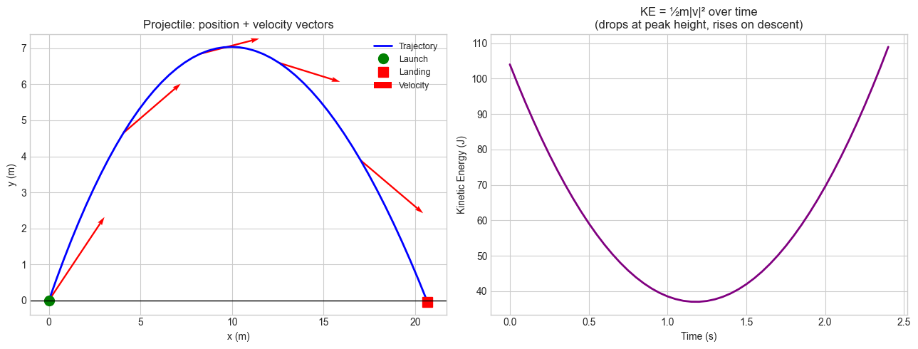
6. Experiments
# --- Experiment 1: Optimal launch angle ---
# Hypothesis: Maximum range is achieved at 45° (no air resistance).
# With wind, the optimal angle shifts.

import numpy as np
import matplotlib.pyplot as plt

plt.style.use('seaborn-v0_8-whitegrid')

SPEED = 15.0    # launch speed (m/s)  <-- modify
WIND_X = 0.0    # horizontal wind force (N)  <-- try 2.0

angles = np.linspace(5, 85, 80)
ranges = []

for deg in angles:
    theta = np.radians(deg)
    p = Particle(1.0, [0.,0.], [SPEED*np.cos(theta), SPEED*np.sin(theta)])
    for _ in range(2000):
        if p.x[1] < 0 and len(p.history_x) > 5:
            break
        p.apply_forces([np.array([WIND_X, -9.81]), ], 0.02)
    ranges.append(p.x[0])

best_angle = angles[np.argmax(ranges)]
fig, ax = plt.subplots(figsize=(8, 4))
ax.plot(angles, ranges, 'b-', lw=2)
ax.axvline(best_angle, color='red', linestyle='--', label=f'Best angle = {best_angle:.1f}°')
ax.axvline(45, color='gray', linestyle=':', label='45° (no-wind optimum)')
ax.set_xlabel('Launch angle (degrees)')
ax.set_ylabel('Range (m)')
ax.set_title(f'Range vs launch angle (wind={WIND_X} N, speed={SPEED} m/s)')
ax.legend()
plt.tight_layout()
plt.show()
print(f"Optimal angle: {best_angle:.1f}° (max range: {max(ranges):.2f} m)")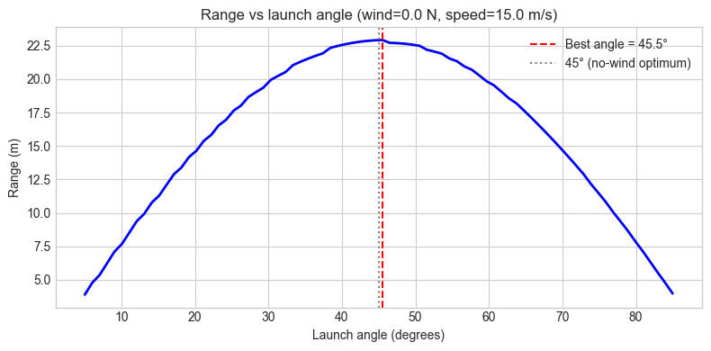
Optimal angle: 45.5° (max range: 22.92 m)
# --- Experiment 2: Work done by a force along a curved path ---
# Hypothesis: Work = F · total displacement (for constant F),
# regardless of the path taken.

import numpy as np

F = np.array([3.0, 1.5])   # constant force  <-- modify

# Path 1: straight line from A to B
A = np.array([0., 0.])
B = np.array([4., 2.])
d_straight = B - A
W_straight = F @ d_straight

# Path 2: via intermediate point C
C = np.array([1., 3.])
W_via_C = F @ (C - A) + F @ (B - C)

# Path 3: many random waypoints
rng = np.random.default_rng(42)
waypoints = np.vstack([A, rng.uniform(0,4,(8,2)), B])
W_random = sum(F @ (waypoints[i+1] - waypoints[i]) for i in range(len(waypoints)-1))

print("Work done by constant force F = (3, 1.5) from A=(0,0) to B=(4,2):")
print(f"  Straight path:      W = {W_straight:.4f} J")
print(f"  Via point C:        W = {W_via_C:.4f} J")
print(f"  Random waypoints:   W = {W_random:.4f} J")
print()
print("All equal — constant force is a conservative field.")
print("Work depends only on start and end points, not the path.")
Work done by constant force F = (3, 1.5) from A=(0,0) to B=(4,2):
Straight path: W = 15.0000 J
Via point C: W = 15.0000 J
Random waypoints: W = 15.0000 J
All equal — constant force is a conservative field.
Work depends only on start and end points, not the path.
7. Exercises
Easy 1. Three forces act on an object: F₁ = (2, 3), F₂ = (−1, 4), F₃ = (0, −5). Find the net force and its magnitude. If the object has mass 2 kg, what is its acceleration vector?
Easy 2. Compute the work done by force F = (5, 2, −1) N over displacement d = (3, 0, 4) m. Is the force doing positive or negative work along the z-axis component?
Medium 1. Simulate a particle starting at (0, 5) m with velocity (2, 0) m/s under gravity only (no wind). Plot the trajectory. Compare with the analytic solution x(t) = x₀ + v₀t + ½at².
Medium 2. A wrench of length r = (0.3, 0, 0) m applies force F = (0, 50, 0) N to a bolt. Compute the torque vector. What is its magnitude (turning force in N·m)? Which direction does the bolt turn?
Hard. Implement a 2D two-body gravity simulation: two particles attract each other with force F = G·m₁·m₂/|r|² directed along the line connecting them. Simulate for 500 steps and plot both trajectories. Verify conservation of total momentum (p₁ + p₂ = const).
8. Mini Project
# --- Mini Project: Bouncing Ball Simulator ---
#
# Simulate a ball under gravity that bounces off walls.
# Track energy to see how numerical integration loses it over time.

import numpy as np
import matplotlib.pyplot as plt

plt.style.use('seaborn-v0_8-whitegrid')

MASS = 1.0
DT = 0.03
N_STEPS = 600
RESTITUTION = 0.85   # energy kept per bounce  <-- try 1.0 (elastic), 0.5
BOX = np.array([[-5., 5.], [0., 8.]])  # [[xmin,xmax],[ymin,ymax]]

x = np.array([0., 5.0])
v = np.array([3.5, 4.0])
gravity = np.array([0., -9.81 * MASS])

traj = [x.copy()]
energies = [0.5*MASS*(v@v) + MASS*9.81*x[1]]
bounce_count = 0

for _ in range(N_STEPS):
    a = gravity / MASS
    v = v + a * DT
    x = x + v * DT

    # Boundary collisions
    for dim in range(2):
        if x[dim] < BOX[dim, 0]:
            x[dim] = BOX[dim, 0]
            v[dim] = abs(v[dim]) * RESTITUTION
            bounce_count += 1
        elif x[dim] > BOX[dim, 1]:
            x[dim] = BOX[dim, 1]
            v[dim] = -abs(v[dim]) * RESTITUTION
            bounce_count += 1

    traj.append(x.copy())
    energies.append(0.5*MASS*(v@v) + MASS*9.81*x[1])

traj = np.array(traj)
energies = np.array(energies)

fig, (ax1, ax2) = plt.subplots(1, 2, figsize=(12, 5))

# Trajectory colored by speed
speeds = np.linalg.norm(np.diff(traj, axis=0) / DT, axis=1)
sc = ax1.scatter(traj[:-1,0], traj[:-1,1], c=speeds, cmap='hot', s=4)
plt.colorbar(sc, ax=ax1, label='Speed (m/s)')
rect = plt.Rectangle((BOX[0,0], BOX[1,0]),
                       BOX[0,1]-BOX[0,0], BOX[1,1]-BOX[1,0],
                       fill=False, edgecolor='blue', lw=2)
ax1.add_patch(rect)
ax1.set_xlabel('x (m)'); ax1.set_ylabel('y (m)')
ax1.set_title(f'Bouncing ball trajectory\n{bounce_count} bounces, restitution={RESTITUTION}')

# Energy over time
ax2.plot(np.arange(len(energies))*DT, energies, 'purple', lw=1.5)
ax2.set_xlabel('Time (s)'); ax2.set_ylabel('Total energy (J)')
ax2.set_title(f'Energy decay: {energies[0]:.2f} → {energies[-1]:.2f} J\n'
               f'(restitution={RESTITUTION} → energy loss per bounce)')

plt.tight_layout()
plt.show()
9. Chapter Summary & Connections
What was covered:
Physical quantities with magnitude and direction are vectors; they obey the same algebra as abstract vectors.
Force superposition = vector addition. Newton’s second law is a vector equation.
Work = dot product of force and displacement (scalar — the component along motion).
Torque = cross product of position and force (vector — rotation axis and magnitude).
Euler integration is a per-timestep scalar multiplication and vector addition.
Backward connection: The dot product (introduced in ch131) and cross product (introduced in ch136) find their most tangible physical meaning here. The projection formula (introduced in ch134) gives the exact component of force that does work.
Forward connections:
In ch149 (Project: Particle Simulation), these mechanics are extended to multi-particle systems with interaction forces.
This will reappear in ch213 (Gradient Intuition): gradients are force-like vectors pointing in the direction of steepest increase — gradient descent is anti-gravity for a loss landscape.
In ch150 (Project: Vector-Based Game Physics), the full rigid-body simulation pipeline uses everything in this chapter simultaneously.