Prerequisites: ch131 (Dot Product), ch128 (Norm), ch129 (Distance), ch133 (Angles), ch134 (Projections), ch127 (Linear Combination)
You will learn:
How data points, feature vectors, and model parameters are all vectors
How similarity, distance, and angle between vectors power core ML algorithms
How a linear model is a dot product; how a neuron is a dot product + nonlinearity
How vector arithmetic on embeddings encodes semantic meaning
How the geometry of high-dimensional vector spaces shapes ML behavior
Environment: Python 3.x, numpy, matplotlib
1. Concept
In machine learning, virtually everything is a vector:
A data point is a vector of feature values: x = (age, income, height, ...) ∈ ℝⁿ
A model parameter set is a vector: w ∈ ℝⁿ (weights), b ∈ ℝ (bias)
A word embedding is a vector: “king” → e ∈ ℝ³⁰⁰
A neural network layer is a linear transformation of its input vector
Predictions are dot products: ŷ = w · x + b
Loss gradients are vectors pointing in the direction of steepest parameter change
Every operation in ML reduces to vector operations: addition, scalar multiplication, dot products, norms, and matrix-vector products. Understanding vectors is not background — it is the core.
Common misconception: “Feature engineering is domain-specific; vectors are just storage.” Wrong — the geometric relationships between feature vectors (distance, angle, projection) determine what the model can and cannot learn.
2. Intuition & Mental Models
Data as points in space: Each data sample is a point in n-dimensional feature space. Classification draws boundaries between clusters of points. Regression finds a hyperplane passing through the cloud. The geometry of the cloud determines difficulty.
Prediction as dot product: A linear model computes ŷ = w · x. Geometrically, this is the projection of x onto w, scaled by ‖w‖. The sign of the dot product determines which side of the decision boundary x falls on. (Projection, introduced in ch134.)
Cosine similarity: Two feature vectors with small angle between them (large cosine similarity) represent similar samples. This is more robust than Euclidean distance in high dimensions because it ignores magnitude — a common technique in text and recommendation systems. (Angles, introduced in ch133.)
Embedding arithmetic: In word2vec-style embeddings, semantic relationships are encoded as vector differences: e(king) − e(man) ≈ e(queen) − e(woman). Addition and subtraction on embedding vectors correspond to semantic composition.
3. Visualization
# --- Visualization: Feature space geometry and linear classification ---

import numpy as np
import matplotlib.pyplot as plt

plt.style.use('seaborn-v0_8-whitegrid')
rng = np.random.default_rng(42)

fig, axes = plt.subplots(1, 3, figsize=(15, 5))

# --- Panel 1: Data as vectors in feature space ---
ax = axes[0]
# Two classes
class0 = rng.multivariate_normal([2,2], [[0.5,0.2],[0.2,0.5]], 30)
class1 = rng.multivariate_normal([4,4], [[0.5,-0.1],[-0.1,0.5]], 30)
ax.scatter(*class0.T, c='blue', s=30, label='Class 0', alpha=0.7)
ax.scatter(*class1.T, c='red', s=30, label='Class 1', alpha=0.7)
# Show one sample as a vector from origin
sample = class0[5]
ax.annotate('', xy=sample, xytext=[0,0],
            arrowprops=dict(arrowstyle='->', color='purple', lw=2))
ax.text(sample[0]/2-0.3, sample[1]/2+0.2, 'x = feature vector', fontsize=9, color='purple')
ax.set_xlabel('Feature 1'); ax.set_ylabel('Feature 2')
ax.set_title('Data points as vectors in feature space')
ax.legend(fontsize=9)
ax.axhline(0, color='k', lw=0.5); ax.axvline(0, color='k', lw=0.5)

# --- Panel 2: Linear classifier as dot product ---
ax2 = axes[1]
# Weight vector defines the normal to the decision boundary
w = np.array([1.0, 1.0])  # weight vector
b = -5.5                   # bias

ax2.scatter(*class0.T, c='blue', s=30, alpha=0.7)
ax2.scatter(*class1.T, c='red', s=30, alpha=0.7)

# Decision boundary: w·x + b = 0  =>  x2 = -(w1*x1 + b)/w2
x1_vals = np.linspace(0, 6, 100)
x2_boundary = -(w[0]*x1_vals + b) / w[1]
ax2.plot(x1_vals, x2_boundary, 'k-', lw=2, label='Decision boundary\n(w·x + b = 0)')

# Weight vector (normal to boundary)
mid = np.array([3.0, -(w[0]*3.0+b)/w[1]])
ax2.annotate('', xy=mid+w*0.6, xytext=mid,
             arrowprops=dict(arrowstyle='->', color='green', lw=2.5))
ax2.text(mid[0]+w[0]*0.65, mid[1]+w[1]*0.65, 'w', fontsize=14, color='green')
ax2.set_xlim(0, 6); ax2.set_ylim(0, 6)
ax2.set_xlabel('Feature 1'); ax2.set_ylabel('Feature 2')
ax2.set_title('Linear classifier: ŷ = sign(w·x + b)\nw is normal to decision boundary')
ax2.legend(fontsize=9)

# --- Panel 3: Cosine similarity heatmap ---
ax3 = axes[2]
# Sample 8 data points and compute pairwise cosine similarity
pts = np.vstack([class0[:4], class1[:4]])
norms = np.linalg.norm(pts, axis=1, keepdims=True)
pts_normed = pts / norms
cos_sim = pts_normed @ pts_normed.T

im = ax3.imshow(cos_sim, cmap='RdYlGn', vmin=-1, vmax=1)
plt.colorbar(im, ax=ax3)
ax3.set_xticks(range(8))
ax3.set_yticks(range(8))
labels = [f'C0_{i}' for i in range(4)] + [f'C1_{i}' for i in range(4)]
ax3.set_xticklabels(labels, fontsize=8, rotation=45)
ax3.set_yticklabels(labels, fontsize=8)
ax3.set_title('Cosine similarity matrix\n(same class = higher similarity)')

plt.tight_layout()
plt.show()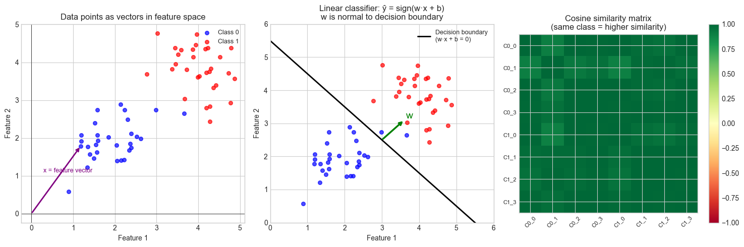
4. Mathematical Formulation
Linear model (regression):
ŷ = w · x + b = wᵀx + bwhere w ∈ ℝⁿ (weights), b ∈ ℝ (bias), x ∈ ℝⁿ (features). This is a dot product — the projection of x onto w, scaled and shifted.
Linear classifier:
ŷ = sign(w · x + b)The decision boundary is the hyperplane {x : w · x + b = 0}. The weight vector w is normal to this hyperplane.
Neuron (single):
output = σ(w · x + b)where σ is a non-linear activation function (sigmoid, ReLU, etc.). The linear part is a dot product; the non-linearity is applied after.
Cosine similarity:
cos_sim(x, y) = (x · y) / (||x|| · ||y||) ∈ [−1, 1]Used in: nearest-neighbor search, recommendation systems, NLP similarity.
k-NN distance:
distance(x, xᵢ) = ||x - xᵢ||₂The k nearest neighbors are the k training points with smallest distance to x.
Embedding arithmetic (word2vec):
e(king) - e(man) + e(woman) ≈ e(queen)Semantic relationships = vector arithmetic in embedding space.
Batch prediction (matrix form):
ŷ = Xw + bwhere X is the data matrix (N samples × n features). This is a matrix-vector product, covered in ch151+.
5. Python Implementation
# --- Implementation: Core ML vector operations from scratch ---

import numpy as np


def cosine_similarity(a, b):
    """
    Cosine similarity between vectors a and b.
    Returns scalar in [-1, 1].
    """
    return float(np.dot(a, b) / (np.linalg.norm(a) * np.linalg.norm(b) + 1e-12))


def cosine_similarity_matrix(X):
    """
    Pairwise cosine similarity for all rows of X.

    Args:
        X: np.ndarray, shape (N, d)

    Returns:
        np.ndarray, shape (N, N)
    """
    norms = np.linalg.norm(X, axis=1, keepdims=True)
    X_normed = X / (norms + 1e-12)
    return X_normed @ X_normed.T


def linear_predict(X, w, b):
    """
    Linear model prediction: ŷ = Xw + b

    Args:
        X: np.ndarray, shape (N, d)
        w: np.ndarray, shape (d,)
        b: float

    Returns:
        np.ndarray, shape (N,)
    """
    return X @ w + b


def knn_predict(X_train, y_train, X_test, k=3):
    """
    k-nearest neighbors classifier using Euclidean distance.

    Args:
        X_train: np.ndarray, shape (N, d)
        y_train: np.ndarray, shape (N,)  — integer class labels
        X_test:  np.ndarray, shape (M, d)
        k: int — number of neighbors

    Returns:
        np.ndarray, shape (M,) — predicted class labels
    """
    predictions = []
    for x in X_test:
        # Distance from x to each training point
        diffs = X_train - x            # shape (N, d)
        dists = np.linalg.norm(diffs, axis=1)  # shape (N,)
        knn_idx = np.argsort(dists)[:k]
        # Majority vote
        neighbor_labels = y_train[knn_idx]
        pred = np.bincount(neighbor_labels).argmax()
        predictions.append(pred)
    return np.array(predictions)


def sigmoid(z):
    """Sigmoid activation: σ(z) = 1 / (1 + e^{-z})"""
    return 1.0 / (1.0 + np.exp(-z))


# --- Demo: kNN on synthetic 2D data ---
rng = np.random.default_rng(0)
X_train = np.vstack([
    rng.multivariate_normal([1,1], 0.3*np.eye(2), 30),
    rng.multivariate_normal([3,3], 0.3*np.eye(2), 30),
])
y_train = np.array([0]*30 + [1]*30)

X_test = np.array([[2., 2.], [0.5, 1.2], [3.5, 3.5], [1.5, 2.5]])
preds = knn_predict(X_train, y_train, X_test, k=5)

print("k-NN predictions (k=5):")
for x, p in zip(X_test, preds):
    print(f"  x={x}  ->  class {p}")

print()
print("Cosine similarities between test points:")
C = cosine_similarity_matrix(X_test)
print(C.round(3))
k-NN predictions (k=5):
x=[2. 2.] -> class 0
x=[0.5 1.2] -> class 0
x=[3.5 3.5] -> class 1
x=[1.5 2.5] -> class 0
Cosine similarities between test points:
[[1. 0.925 1. 0.97 ]
[0.925 1. 0.925 0.989]
[1. 0.925 1. 0.97 ]
[0.97 0.989 0.97 1. ]]
# --- Embedding arithmetic demo ---
# Simulate word2vec-style embeddings with synthetic vectors

import numpy as np

rng = np.random.default_rng(7)
DIM = 50  # embedding dimension  <-- try 5, 300

# Construct embeddings with built-in analogies
# Gender axis: man-woman, king-queen
gender_axis = rng.standard_normal(DIM)
gender_axis /= np.linalg.norm(gender_axis)

royalty_axis = rng.standard_normal(DIM)
royalty_axis /= np.linalg.norm(royalty_axis)

base = rng.standard_normal(DIM) * 0.3

embeddings = {
    'man':   base + 0.8*gender_axis + rng.standard_normal(DIM)*0.05,
    'woman': base - 0.8*gender_axis + rng.standard_normal(DIM)*0.05,
    'king':  base + 0.8*gender_axis + 1.2*royalty_axis + rng.standard_normal(DIM)*0.05,
    'queen': base - 0.8*gender_axis + 1.2*royalty_axis + rng.standard_normal(DIM)*0.05,
    'prince':base + 0.8*gender_axis + 0.9*royalty_axis + rng.standard_normal(DIM)*0.05,
    'cat':   rng.standard_normal(DIM),  # unrelated word
}

def closest(query_vec, embeddings, top_k=3):
    """Find top-k words by cosine similarity to query_vec."""
    sims = {word: cosine_similarity(query_vec, vec)
            for word, vec in embeddings.items()}
    return sorted(sims.items(), key=lambda x: -x[1])[:top_k]

# king - man + woman ≈ queen
query = embeddings['king'] - embeddings['man'] + embeddings['woman']
print("king - man + woman -> closest words:")
for word, sim in closest(query, embeddings):
    print(f"  {word:10s}  cos_sim = {sim:.4f}")

print()
# Gender analogy
print("Cosine similarity, king vs queen:",
      round(cosine_similarity(embeddings['king'], embeddings['queen']), 4))
print("Cosine similarity, king vs cat:  ",
      round(cosine_similarity(embeddings['king'], embeddings['cat']), 4))
king - man + woman -> closest words:
queen cos_sim = 0.9550
woman cos_sim = 0.8303
king cos_sim = 0.7495
Cosine similarity, king vs queen: 0.7187
Cosine similarity, king vs cat: 0.1441
6. Experiments
# --- Experiment 1: Curse of dimensionality — distances collapse ---
# Hypothesis: In high dimensions, all pairwise distances become similar.
# This is why kNN degrades in high dimensions.

import numpy as np
import matplotlib.pyplot as plt

plt.style.use('seaborn-v0_8-whitegrid')

rng = np.random.default_rng(0)
DIMS = [2, 5, 10, 50, 100, 500, 1000]  # <-- modify
N = 200

ratios = []
for d in DIMS:
    X = rng.standard_normal((N, d))
    # Pairwise distances
    diffs = X[:, None, :] - X[None, :, :]  # (N, N, d)
    dists = np.linalg.norm(diffs, axis=-1)  # (N, N)
    upper = dists[np.triu_indices(N, k=1)]
    ratios.append((upper.max() - upper.min()) / upper.mean())

fig, ax = plt.subplots(figsize=(8, 4))
ax.semilogx(DIMS, ratios, 'bo-', lw=2, markersize=8)
ax.set_xlabel('Dimension')
ax.set_ylabel('(max−min) / mean distance')
ax.set_title('Curse of dimensionality: distances become indistinguishable\n'
              'as dimension grows (ratio → 0)')
plt.tight_layout()
plt.show()

print(f"{'Dim':>6}  {'(max-min)/mean':>16}")
for d, r in zip(DIMS, ratios):
    print(f"  {d:4d}  {r:16.4f}")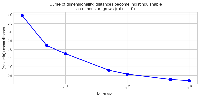
   Dim    (max-min)/mean
     2            3.9596
     5            2.2152
    10            1.7616
    50            0.8043
   100            0.5737
   500            0.2660
  1000            0.1937
# --- Experiment 2: Decision boundary = dot product threshold ---
# Visualize how different weight vectors create different decision boundaries.

import numpy as np
import matplotlib.pyplot as plt

plt.style.use('seaborn-v0_8-whitegrid')

rng = np.random.default_rng(3)
X = np.vstack([
    rng.multivariate_normal([1,1], 0.4*np.eye(2), 40),
    rng.multivariate_normal([3,3], 0.4*np.eye(2), 40),
])
y = np.array([0]*40 + [1]*40)

weight_vectors = [
    (np.array([1.0, 1.0]), -3.5, 'w=(1,1)'),
    (np.array([1.0, 0.0]), -2.0, 'w=(1,0) — uses feature 1 only'),
    (np.array([0.5, 1.5]), -4.0, 'w=(0.5,1.5) — upweights feature 2'),
]  # <-- modify weights and biases

fig, axes = plt.subplots(1, 3, figsize=(13, 4))
x1_range = np.linspace(-0.5, 5, 100)

for ax, (w, b, title) in zip(axes, weight_vectors):
    ax.scatter(*X[y==0].T, c='blue', s=25, alpha=0.7, label='Class 0')
    ax.scatter(*X[y==1].T, c='red', s=25, alpha=0.7, label='Class 1')

    # Decision boundary: w[0]*x1 + w[1]*x2 + b = 0
    if abs(w[1]) > 1e-9:
        x2_boundary = -(w[0]*x1_range + b) / w[1]
        ax.plot(x1_range, x2_boundary, 'k-', lw=2)

    # Weight vector
    cx, cy = 2.0, 2.0
    ax.annotate('', xy=(cx+w[0]*0.5, cy+w[1]*0.5), xytext=(cx, cy),
                arrowprops=dict(arrowstyle='->', color='green', lw=2.5))

    preds = np.sign(X @ w + b)
    acc = np.mean(preds == (2*y - 1))
    ax.set_title(f'{title}\naccuracy={acc:.0%}', fontsize=9)
    ax.set_xlim(-0.5, 5); ax.set_ylim(-0.5, 5)
    ax.legend(fontsize=8)

plt.suptitle('Decision boundary determined by weight vector direction', fontsize=11)
plt.tight_layout()
plt.show()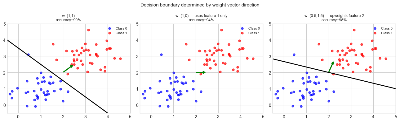
7. Exercises
Easy 1. Given weight vector w = (2, −1, 0.5) and bias b = −1, compute the linear model prediction for x = (1, 3, 2). Is the prediction positive or negative? What class does it predict?
Easy 2. Compute the cosine similarity between a = (1, 2, 3) and b = (3, 2, 1). Are they similar? What about a and c = (−1, −2, −3)?
Medium 1. Implement a function document_similarity(doc1_tfidf, doc2_tfidf) that uses cosine similarity on TF-IDF-like vectors. Generate three synthetic “documents” as sparse vectors and find which pair is most similar.
Medium 2. Implement k-NN classification using cosine distance instead of Euclidean distance. On the same 2D synthetic dataset, compare the decision boundaries. When does cosine distance perform better?
Hard. Implement logistic regression from scratch using only vector operations: (a) prediction: σ(w·x + b), (b) binary cross-entropy loss, (c) gradient computation via dot products, (d) gradient descent update. Train it on the 2D synthetic dataset and plot the learning curve and decision boundary.
8. Mini Project
# --- Mini Project: Vector-Based Recommendation Engine ---
#
# Problem: Represent users and items as vectors. Recommend items
# whose vectors are most similar to a user's preference vector.
# This is the foundation of collaborative filtering.

import numpy as np
import matplotlib.pyplot as plt

plt.style.use('seaborn-v0_8-whitegrid')
rng = np.random.default_rng(0)

# --- Setup: items and users in 3D "taste space" ---
# Dimensions: [action, drama, comedy]
ITEMS = {
    'Die Hard':       np.array([0.95, 0.2, 0.1]),
    'The Notebook':   np.array([0.1, 0.9, 0.3]),
    'Superbad':       np.array([0.1, 0.1, 0.95]),
    'Mad Max':        np.array([0.9, 0.3, 0.05]),
    'Schindlers List':np.array([0.1, 0.95, 0.05]),
    'Anchorman':      np.array([0.05, 0.05, 0.9]),
    'Heat':           np.array([0.85, 0.5, 0.1]),
    'When Harry Met': np.array([0.05, 0.6, 0.8]),
}

# User preference vectors (from their viewing history)
USERS = {
    'Alice':  np.array([0.8, 0.2, 0.1]),   # loves action
    'Bob':    np.array([0.1, 0.1, 0.9]),   # loves comedy
    'Carol':  np.array([0.3, 0.8, 0.4]),   # loves drama + some comedy
}

# Normalize all vectors
def normalize(v):
    return v / (np.linalg.norm(v) + 1e-12)

items_norm = {k: normalize(v) for k, v in ITEMS.items()}
users_norm = {k: normalize(v) for k, v in USERS.items()}

def recommend(user_name, top_k=3):
    """Recommend top-k items for a user using cosine similarity."""
    u = users_norm[user_name]
    scores = {item: float(u @ iv) for item, iv in items_norm.items()}
    ranked = sorted(scores.items(), key=lambda x: -x[1])
    return ranked[:top_k]

print("Recommendations:")
for user in USERS:
    recs = recommend(user)
    print(f"\n{user} (preferences: {USERS[user]}):")
    for item, score in recs:
        print(f"  {item:20s}  similarity = {score:.4f}")

# --- Visualization in 3D taste space ---
from mpl_toolkits.mplot3d import Axes3D

fig = plt.figure(figsize=(9, 7))
ax = fig.add_subplot(111, projection='3d')

for name, v in ITEMS.items():
    ax.scatter(*v, c='steelblue', s=80, zorder=5)
    ax.text(v[0]+0.02, v[1]+0.02, v[2]+0.02, name, fontsize=8)

colors = ['red', 'green', 'purple']
for (name, v), c in zip(USERS.items(), colors):
    ax.quiver(0, 0, 0, *v, color=c, lw=2.5, arrow_length_ratio=0.15)
    ax.text(*v*1.05, name, fontsize=10, color=c, fontweight='bold')

ax.set_xlabel('Action'); ax.set_ylabel('Drama'); ax.set_zlabel('Comedy')
ax.set_title('3D Taste Space: items (blue) and user preferences (arrows)')
plt.tight_layout()
plt.show()
9. Chapter Summary & Connections
What was covered:
Data, parameters, and predictions are all vectors; ML operations are vector operations.
Linear prediction = dot product. The decision boundary is the hyperplane normal to w.
Cosine similarity measures directional alignment — robust to magnitude differences.
k-NN uses Euclidean distance (vector norms); degrades in high dimensions (curse of dimensionality).
Embedding arithmetic (word2vec-style) encodes semantic relationships as vector geometry.
Backward connection: Every concept in this chapter is a direct application of ch128–134 (norms, distances, dot products, angles, projections). The math was not abstract preparation — it was the exact vocabulary ML uses.
Forward connections:
In ch188 (Linear Layers in Deep Learning), a layer is Xw + b for a batch X — a matrix operation extending the dot product to many samples simultaneously.
This will reappear in ch185 (PCA Intuition): principal components are the directions that explain maximum variance — eigenvectors of the data covariance matrix.
In ch295–300 (Part IX capstone), the full ML pipeline — features, model, loss, optimization — is assembled using all the vector tools from this part.