Prerequisites: Matrix representation (ch152), vector addition (ch125)
You will learn:
Matrix addition as elementwise operation
Scalar multiplication of matrices
Broadcasting in NumPy
What matrix addition means geometrically (combining transformations)
Environment: Python 3.x, numpy, matplotlib
1. Concept
Matrix addition is the simplest matrix operation: add corresponding entries. Two matrices can be added only if they have the same shape.
This is structurally identical to vector addition (ch125) — a matrix is just a vector that happens to be arranged in two dimensions.
More importantly: adding two transformation matrices gives a transformation that is the sum of the two transformations. This is a direct consequence of linearity.
Common misconceptions:
“You can add any two matrices.” — Only if they have identical shape.
“Matrix addition and matrix multiplication are similar operations.” — They are not. Addition is elementwise and commutative; multiplication is not.
2. Intuition & Mental Models
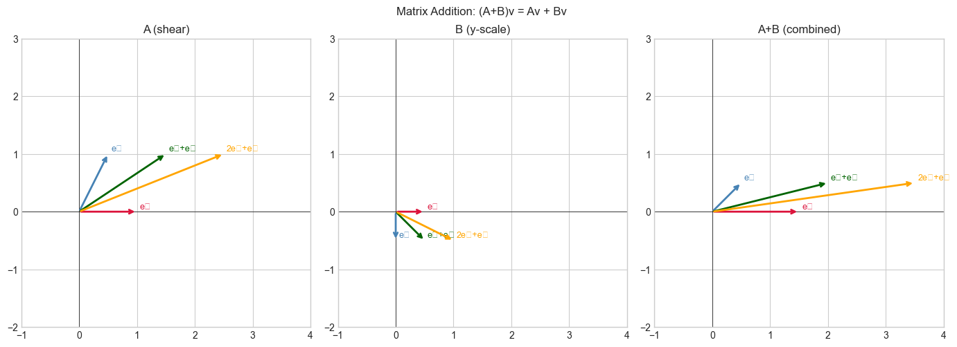
Geometric: If A stretches the x-axis and B rotates, then A+B is a new transformation that does both effects simultaneously, applied to each basis vector independently. The output of (A+B)v equals Av + Bv — both transformations applied and summed.
Computational: Think of matrix addition as a vectorized for-loop over all entries. C[i,j] = A[i,j] + B[i,j] for every (i,j).
Recall from ch125 (Vector Addition) that adding vectors is tip-to-tail. Matrix addition is the same thing — but done simultaneously for every row of each matrix considered as a vector.
3. Visualization
# --- Visualization: (A+B)v = Av + Bv ---
import numpy as np
import matplotlib.pyplot as plt
plt.style.use('seaborn-v0_8-whitegrid')

A = np.array([[1.0, 0.5], [0.0, 1.0]])   # shear
B = np.array([[0.5, 0.0], [0.0, -0.5]])  # scale y by -0.5
C = A + B

# Test vectors
vectors = np.array([[1,0],[0,1],[1,1],[2,1]], dtype=float).T  # 2x4

Av = A @ vectors
Bv = B @ vectors
Cv = C @ vectors
AvpBv = Av + Bv   # should equal Cv

print("Verifying (A+B)v = Av + Bv for all test vectors:")
print(f"Max difference: {np.max(np.abs(Cv - AvpBv)):.2e}")

fig, axes = plt.subplots(1, 3, figsize=(14, 5))
colors = ['crimson','steelblue','darkgreen','orange']
labels = ['e₁','e₂','e₁+e₂','2e₁+e₂']

for ax, mat, title in zip(axes, [A, B, C], ['A (shear)', 'B (y-scale)', 'A+B (combined)']):
    result = mat @ vectors
    for k in range(vectors.shape[1]):
        ax.annotate('', xy=result[:,k], xytext=(0,0),
                    arrowprops=dict(arrowstyle='->', color=colors[k], lw=2))
        ax.text(result[0,k]+0.05, result[1,k]+0.05, labels[k], fontsize=9, color=colors[k])
    ax.set_xlim(-1, 4); ax.set_ylim(-2, 3); ax.set_aspect('equal')
    ax.axhline(0, color='k', lw=0.5); ax.axvline(0, color='k', lw=0.5)
    ax.set_title(title)

plt.suptitle('Matrix Addition: (A+B)v = Av + Bv', fontsize=12)
plt.tight_layout()
plt.show()
Verifying (A+B)v = Av + Bv for all test vectors:
Max difference: 0.00e+00
C:\Users\user\AppData\Local\Temp\ipykernel_13560\2149386769.py:36: UserWarning: Glyph 8321 (\N{SUBSCRIPT ONE}) missing from font(s) Arial.
  plt.tight_layout()
C:\Users\user\AppData\Local\Temp\ipykernel_13560\2149386769.py:36: UserWarning: Glyph 8322 (\N{SUBSCRIPT TWO}) missing from font(s) Arial.
  plt.tight_layout()
c:\Users\user\OneDrive\Documents\book\.venv\Lib\site-packages\IPython\core\pylabtools.py:170: UserWarning: Glyph 8321 (\N{SUBSCRIPT ONE}) missing from font(s) Arial.
  fig.canvas.print_figure(bytes_io, **kw)
c:\Users\user\OneDrive\Documents\book\.venv\Lib\site-packages\IPython\core\pylabtools.py:170: UserWarning: Glyph 8322 (\N{SUBSCRIPT TWO}) missing from font(s) Arial.
  fig.canvas.print_figure(bytes_io, **kw)
4. Mathematical Formulation
Matrix addition (A, B same shape m×n):
  (A + B)[i,j] = A[i,j] + B[i,j]   for all i, j

Scalar multiplication:
  (αA)[i,j] = α * A[i,j]            for all i, j

Key properties:
  Commutativity:    A + B = B + A
  Associativity:    (A+B)+C = A+(B+C)
  Zero matrix:      A + 0 = A  (0 is the m×n zero matrix)
  Distributivity:   α(A+B) = αA + αB
  Linearity proof:  (A+B)v = Av + Bv  (follows directly from distributivity of dot product)
# --- Implementation: Matrix arithmetic from scratch and with NumPy ---
import numpy as np
def matrix_add(A, B):
"""
Add two matrices elementwise.
Args:
A, B: 2D numpy arrays of the same shape
Returns:
C: 2D numpy array, A + B
"""
if A.shape != B.shape:
raise ValueError(f"Shape mismatch: {A.shape} vs {B.shape}")
m, n = A.shape
C = np.empty((m, n), dtype=float)
for i in range(m):
for j in range(n):
C[i, j] = A[i, j] + B[i, j]
return C
def scalar_mult(alpha, A):
"""
Multiply matrix A by scalar alpha.
Args:
alpha: scalar
A: 2D numpy array
Returns:
2D numpy array, alpha * A
"""
return np.vectorize(lambda x: alpha * x)(A)
# Test
A = np.array([[1, 2], [3, 4]], dtype=float)
B = np.array([[5, -1], [0, 2]], dtype=float)
C_scratch = matrix_add(A, B)
C_numpy = A + B
print(f"From scratch: {C_scratch}")
print(f"NumPy A+B: {C_numpy}")
print(f"Match: {np.allclose(C_scratch, C_numpy)}")
print()
# Broadcasting: add a vector to every row of a matrix
A = np.array([[1,2,3],[4,5,6],[7,8,9]], dtype=float)
bias = np.array([10.0, 0.0, -10.0]) # shape (3,) — broadcasts over rows
print(f"A + bias (broadcast over rows):\n{A + bias}")
# Add a column vector to every column
col_bias = np.array([[100.0], [0.0], [-100.0]]) # shape (3,1)
print(f"\nA + col_bias (broadcast over columns):\n{A + col_bias}")From scratch: [[6. 1.]
[3. 6.]]
NumPy A+B: [[6. 1.]
[3. 6.]]
Match: True
A + bias (broadcast over rows):
[[11. 2. -7.]
[14. 5. -4.]
[17. 8. -1.]]
A + col_bias (broadcast over columns):
[[101. 102. 103.]
[ 4. 5. 6.]
[-93. -92. -91.]]
5. Python Implementation — Broadcasting Rules
# --- Broadcasting: the general rules ---
import numpy as np

# Rule: shapes are compared right-to-left.
# Dimensions are compatible if: equal, or one of them is 1.
# If compatible, the smaller dimension is 'stretched' to match.

examples = [
    (np.ones((3,4)),   np.ones((4,)),    "(3,4) + (4,)   → (3,4)"),
    (np.ones((3,1)),   np.ones((1,4)),   "(3,1) + (1,4)  → (3,4)"),
    (np.ones((5,3,4)), np.ones((3,4)),   "(5,3,4)+(3,4)  → (5,3,4)"),
]

for A, B, desc in examples:
    C = A + B
    print(f"{desc}  result shape: {C.shape}")

# Failure case
try:
    _ = np.ones((3,4)) + np.ones((3,))
except ValueError as e:
    print(f"\n(3,4) + (3,) → Error: {e}")

print("\nML context: adding a bias vector (shape [output_dim]) to a batch")
print("of activations (shape [batch, output_dim]) uses broadcasting.")
batch_size, output_dim = 32, 10
activations = np.random.randn(batch_size, output_dim)
bias = np.random.randn(output_dim)                    # shape (10,)
result = activations + bias                            # broadcasts over batch
print(f"activations {activations.shape} + bias {bias.shape} → {result.shape}")
(3,4) + (4,) → (3,4) result shape: (3, 4)
(3,1) + (1,4) → (3,4) result shape: (3, 4)
(5,3,4)+(3,4) → (5,3,4) result shape: (5, 3, 4)
(3,4) + (3,) → Error: operands could not be broadcast together with shapes (3,4) (3,)
ML context: adding a bias vector (shape [output_dim]) to a batch
of activations (shape [batch, output_dim]) uses broadcasting.
activations (32, 10) + bias (10,) → (32, 10)
6. Experiments
# --- Experiment: Matrix addition as superposition of effects ---
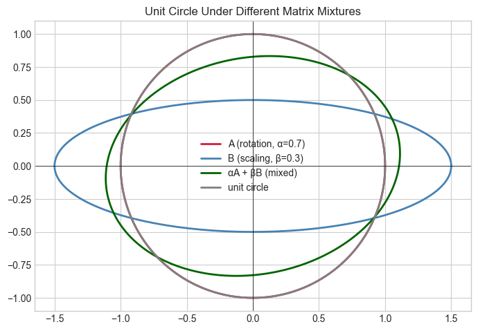
# Hypothesis: Applying A+B to a set of points produces the vector sum of A and B effects.
# Try changing: ALPHA, BETA — the mixing coefficients.
import numpy as np
import matplotlib.pyplot as plt
plt.style.use('seaborn-v0_8-whitegrid')
ALPHA = 0.7 # <-- modify: weight on A (rotation)
BETA = 0.3 # <-- modify: weight on B (scaling)
# A: 30-degree rotation
theta = np.pi / 6
A = np.array([[np.cos(theta), -np.sin(theta)],
[np.sin(theta), np.cos(theta)]])
# B: non-uniform scaling
B = np.array([[1.5, 0.0], [0.0, 0.5]])
# Mix
M = ALPHA * A + BETA * B
# Apply to unit circle
t = np.linspace(0, 2*np.pi, 200)
circle = np.row_stack([np.cos(t), np.sin(t)])
fig, ax = plt.subplots(figsize=(7, 7))
for mat, color, label in [(A, 'crimson', f'A (rotation, α={ALPHA})'),
(B, 'steelblue', f'B (scaling, β={BETA})'),
(M, 'darkgreen', f'αA + βB (mixed)'),
(np.eye(2), 'gray', 'unit circle')]:
result = mat @ circle
ax.plot(result[0], result[1], color=color, label=label, linewidth=2)
ax.set_aspect('equal')
ax.axhline(0, color='k', lw=0.5); ax.axvline(0, color='k', lw=0.5)
ax.legend(); ax.set_title('Unit Circle Under Different Matrix Mixtures')
plt.tight_layout(); plt.show()C:\Users\user\AppData\Local\Temp\ipykernel_13560\1896582526.py:23: DeprecationWarning: `row_stack` alias is deprecated. Use `np.vstack` directly.
circle = np.row_stack([np.cos(t), np.sin(t)])
7. Exercises
Easy 1. Compute A + B by hand: A = [[1,2],[3,4]], B = [[-1,0],[2,-3]]. What is 2A - B?
Easy 2. Why can you not add a (3×4) matrix to a (4×3) matrix? What would you need to do first?
Medium 1. Write a function linear_combo_matrices(matrices, coefficients) that computes a weighted sum of a list of matrices. Use it to interpolate between a rotation matrix and a scaling matrix with α from 0 to 1 in 5 steps. Plot the unit circle under each interpolated matrix.
Medium 2. In a neural network, the forward pass is Z = W @ X + b where W is (m,n), X is (n, batch), and b is (m,). What is the shape of Z? Why does b broadcast correctly here? Write it out.
Hard. Prove that the set of all m×n matrices forms a vector space under matrix addition and scalar multiplication. Identify the zero vector, additive inverse, and verify all 8 axioms with short NumPy demonstrations.
8. Mini Project
# --- Mini Project: Image blending via matrix addition ---
# Problem: Two 'images' (grayscale matrices) should be blended with
# a varying alpha parameter. This is the standard alpha-compositing operation.
# Task: implement blend(A, B, alpha) and show the result for alpha in [0, 0.25, 0.5, 0.75, 1.0]

import numpy as np
import matplotlib.pyplot as plt
plt.style.use('seaborn-v0_8-whitegrid')

SIZE = 64
x = np.linspace(0, 4*np.pi, SIZE)
X, Y = np.meshgrid(x, x)

# Image A: horizontal stripes
img_A = (np.sin(Y * 2) + 1) / 2
# Image B: concentric circles
cx, cy = SIZE//2, SIZE//2
r = np.sqrt((np.arange(SIZE)[:, None] - cy)**2 + (np.arange(SIZE)[None, :] - cx)**2)
img_B = (np.sin(r * 0.5) + 1) / 2

def blend(A, B, alpha):
    """
    Alpha-blend two same-shape matrices.
    alpha=0 → pure A, alpha=1 → pure B.

    Args:
        A, B: 2D numpy arrays (same shape)
        alpha: float in [0, 1]

    Returns:
        2D numpy array
    """
    return (1 - alpha) * A + alpha * B   # pure matrix arithmetic

alphas = [0.0, 0.25, 0.5, 0.75, 1.0]
fig, axes = plt.subplots(1, 5, figsize=(15, 3))
for ax, alpha in zip(axes, alphas):
    blended = blend(img_A, img_B, alpha)
    ax.imshow(blended, cmap='gray', vmin=0, vmax=1)
    ax.set_title(f'α = {alpha}')
    ax.axis('off')

plt.suptitle('Image Alpha Blending: (1-α)A + αB', fontsize=12)
plt.tight_layout()
plt.show()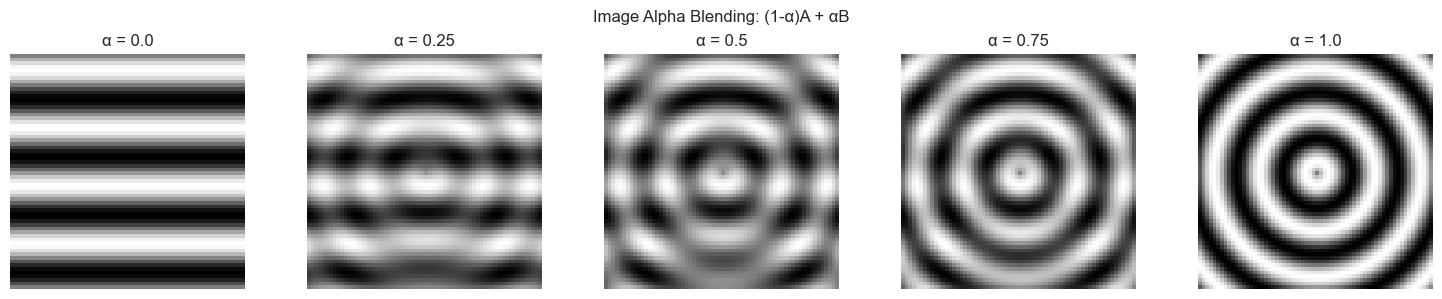
9. Chapter Summary & Connections
Matrix addition is elementwise:
(A+B)[i,j] = A[i,j] + B[i,j]. Shapes must match.(A+B)v = Av + Bv— adding transformation matrices adds their effects on vectors.NumPy broadcasting allows adding matrices with compatible (not necessarily identical) shapes.
The bias term
bin every neural network layer is added via broadcasting (reappears in ch178 — Linear Layers in Deep Learning).
Backward connection: Matrix addition inherits all properties from vector addition (ch125) — matrices are just vectors stored in a 2D grid.
Forward connections:
In ch154 (Matrix Multiplication), we encounter the non-trivial operation — composition, not just elementwise combination.
In ch176 (Matrix Calculus Introduction), the gradient of a scalar-valued matrix function
f(A)is itself a matrix of the same shape — added back to A in gradient descent updates.