Prerequisites: Matrix representation (ch152), matrix addition (ch153), dot product (ch131)
You will learn:
Why matrix multiplication is defined the way it is (composition of transformations)
The three equivalent ways to read a matrix product
Why matrix multiplication is not commutative
How to implement matrix multiplication from scratch
Performance implications: O(n³) naive, O(n^2.37) theoretical
Environment: Python 3.x, numpy, matplotlib
1. Concept
Matrix multiplication is not elementwise. It is function composition.
If B maps vectors from ℝⁿ to ℝᵏ, and A maps vectors from ℝᵏ to ℝᵐ, then AB maps directly from ℝⁿ to ℝᵐ. The product matrix AB is the transformation you get by first applying B, then applying A.
The formula (AB)[i,j] = Σₖ A[i,k] * B[k,j] is the mechanical description. The geometric description: apply B first, then A.
Common misconceptions:
“AB = BA.” — False in general. Order matters: different composition order gives different results.
“The formula is arbitrary.” — It is forced by the requirement that
(AB)v = A(Bv)for all v.“Matrix multiplication is slow.” — NumPy’s
@calls optimized BLAS routines and runs near peak hardware throughput.
2. Intuition & Mental Models
Geometric: Think of AB as a pipeline. You put a vector in, it goes through B, then through A. The resulting matrix encodes the full pipeline in one step.
Computational: Think of (AB)[i,j] as the dot product of row i of A with column j of B. Every output entry is one dot product.
Column view: Each column of AB is A applied to the corresponding column of B. So AB transforms B’s columns by A.
Recall from ch054 (Function Composition) that (f∘g)(x) = f(g(x)). Matrix multiplication is exactly this, but for linear functions.
3. Visualization
# --- Visualization: AB is composition — apply B first, then A ---
import numpy as np
import matplotlib.pyplot as plt
plt.style.use('seaborn-v0_8-whitegrid')

theta = np.pi / 4
# B: rotate 45 degrees
B = np.array([[np.cos(theta), -np.sin(theta)],
              [np.sin(theta),  np.cos(theta)]])
# A: scale x by 2
A = np.array([[2.0, 0.0], [0.0, 1.0]])
# AB: rotate then scale
AB = A @ B
# BA: scale then rotate
BA = B @ A

t = np.linspace(0, 2*np.pi, 300)
circle = np.row_stack([np.cos(t), np.sin(t)])

fig, axes = plt.subplots(1, 4, figsize=(16, 4))
configs = [
    (np.eye(2), 'Original\n(unit circle)'),
    (B,  'B: rotate 45°'),
    (AB, 'AB: rotate THEN scale x2\n(A applied after B)'),
    (BA, 'BA: scale x2 THEN rotate\n(B applied after A)'),
]
for ax, (M, title) in zip(axes, configs):
    result = M @ circle
    ax.plot(result[0], result[1], 'steelblue', lw=2)
    ax.set_xlim(-3, 3); ax.set_ylim(-3, 3)
    ax.set_aspect('equal')
    ax.axhline(0, color='k', lw=0.4); ax.axvline(0, color='k', lw=0.4)
    ax.set_title(title, fontsize=9)

plt.suptitle('AB ≠ BA: Order of Composition Matters', fontsize=13)
plt.tight_layout()
plt.show()

print(f"AB =\n{np.round(AB, 3)}")
print(f"BA =\n{np.round(BA, 3)}")
print(f"AB == BA: {np.allclose(AB, BA)}")
C:\Users\user\AppData\Local\Temp\ipykernel_22640\1242626412.py:18: DeprecationWarning: `row_stack` alias is deprecated. Use `np.vstack` directly.
circle = np.row_stack([np.cos(t), np.sin(t)])
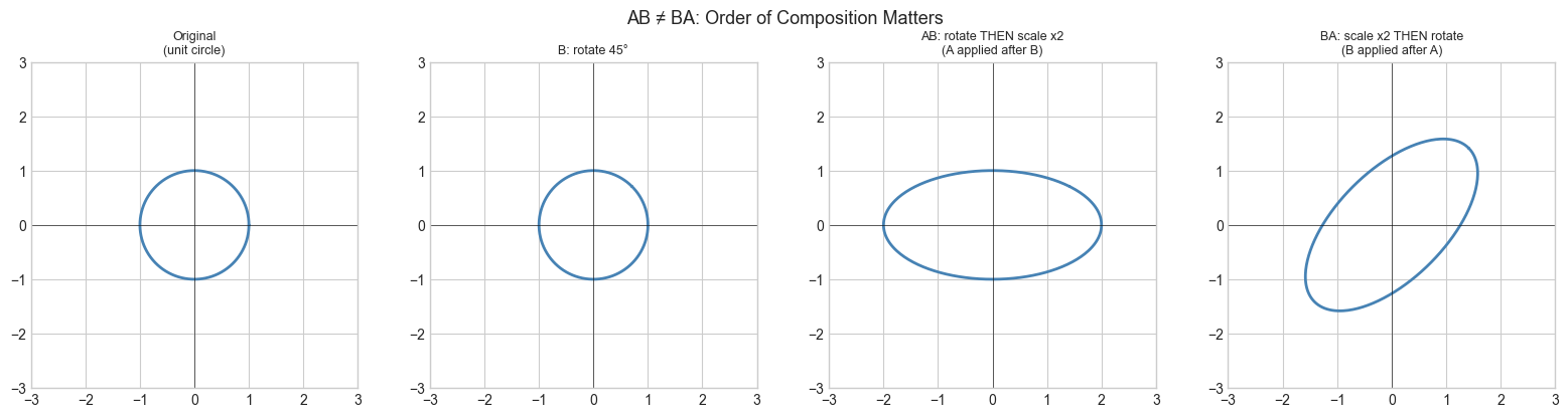
AB =
[[ 1.414 -1.414]
 [ 0.707  0.707]]
BA =
[[ 1.414 -0.707]
 [ 1.414  0.707]]
AB == BA: False
4. Mathematical Formulation
For A (m×k) and B (k×n), the product C = AB is (m×n):

  C[i,j] = Σₗ A[i,l] * B[l,j]   for i=1..m, j=1..n

  ← k terms summed; k is the 'inner dimension' and must match

Three equivalent readings:
  1. C[i,j] = dot(row_i(A), col_j(B))           [row-column dot products]
  2. col_j(C) = A @ col_j(B)                     [A transforms B's columns]
  3. row_i(C) = row_i(A) @ B                     [B transforms A's rows]

Shape rule: (m×k) @ (k×n) = (m×n)   — inner dimensions must match

Associativity: (AB)C = A(BC)         — always true
Commutativity: AB ≠ BA in general    — FALSE for matrices
Distributivity: A(B+C) = AB + AC     — always true
# --- Implementation: Matrix multiplication from scratch (three views) ---
import numpy as np
def matmul_ijk(A, B):
"""
Matrix multiplication: triple-loop (i,j,k) implementation.
Clearest implementation; not fast.
Args:
A: 2D array, shape (m, k)
B: 2D array, shape (k, n)
Returns:
C: 2D array, shape (m, n)
"""
m, k = A.shape
k2, n = B.shape
assert k == k2, f"Inner dims must match: {k} vs {k2}"
C = np.zeros((m, n))
for i in range(m):
for j in range(n):
for l in range(k): # sum over inner dimension
C[i, j] += A[i, l] * B[l, j]
return C
def matmul_dot(A, B):
"""
Matrix multiplication via row-column dot products.
Vectorized over inner dimension.
"""
m, k = A.shape
k2, n = B.shape
assert k == k2
C = np.zeros((m, n))
for i in range(m):
for j in range(n):
C[i, j] = np.dot(A[i, :], B[:, j])
return C
def matmul_col(A, B):
"""
Matrix multiplication via column transformations.
Each column of C = A applied to column of B.
"""
m, k = A.shape
k2, n = B.shape
assert k == k2
C = np.zeros((m, n))
for j in range(n):
C[:, j] = A @ B[:, j] # A applied to column j of B
return C
# Test all three
np.random.seed(42)
A = np.random.randn(4, 3)
B = np.random.randn(3, 5)
C_ijk = matmul_ijk(A, B)
C_dot = matmul_dot(A, B)
C_col = matmul_col(A, B)
C_np = A @ B
print(f"All implementations match: {np.allclose(C_ijk, C_np) and np.allclose(C_dot, C_np) and np.allclose(C_col, C_np)}")
print(f"Output shape: {C_np.shape} (from ({A.shape}) @ ({B.shape}))")All implementations match: True
Output shape: (4, 5) (from ((4, 3)) @ ((3, 5)))
# --- Performance comparison: scratch vs NumPy ---
import numpy as np
import time

N = 200
A = np.random.randn(N, N)
B = np.random.randn(N, N)

# NumPy (BLAS-optimized)
t0 = time.perf_counter()
for _ in range(20): _ = A @ B
t_np = (time.perf_counter() - t0) / 20

# Our column-view implementation
t0 = time.perf_counter()
_ = matmul_col(A, B)
t_scratch = time.perf_counter() - t0

print(f"NumPy @ (N={N}):    {t_np*1000:.3f} ms")
print(f"Scratch matmul_col: {t_scratch*1000:.3f} ms")
print(f"Speedup: {t_scratch/t_np:.0f}x")
print(f"\nNaive: O(N³) = {N**3:,} operations for N={N}")
NumPy @ (N=200): 0.898 ms
Scratch matmul_col: 4.460 ms
Speedup: 5x
Naive: O(N³) = 8,000,000 operations for N=200
6. Experiments
# --- Experiment 1: Non-commutativity ---
# Hypothesis: AB - BA is generally non-zero; but for diagonal matrices it IS zero.
# Try changing: use diagonal matrices and see when AB = BA.
import numpy as np

DIAG = False   # <-- set True to make matrices diagonal

np.random.seed(7)
if DIAG:
    A = np.diag(np.random.randn(3))
    B = np.diag(np.random.randn(3))
else:
    A = np.random.randn(3, 3)
    B = np.random.randn(3, 3)

commutator = A @ B - B @ A   # the 'commutator' [A,B]
print(f"Diagonal mode: {DIAG}")
print(f"||AB - BA||_F = {np.linalg.norm(commutator, 'fro'):.4f}")
print(f"Commute: {np.allclose(A@B, B@A)}")
Diagonal mode: False
||AB - BA||_F = 2.1063
Commute: False
# --- Experiment 2: Chaining transformations ---
# Hypothesis: Rotating by θ twice equals rotating by 2θ. (AB = rotation by 2θ)
# Try changing: THETA, N_REPS
import numpy as np

THETA = np.pi / 6    # <-- 30 degrees
N_REPS = 3           # <-- apply rotation N_REPS times

def rot(theta):
    return np.array([[np.cos(theta), -np.sin(theta)],
                     [np.sin(theta),  np.cos(theta)]])

# Compose N_REPS rotations by THETA
R_single = rot(THETA)
R_composed = np.eye(2)
for _ in range(N_REPS):
    R_composed = R_single @ R_composed

R_direct = rot(N_REPS * THETA)

print(f"Composing rotation(θ={np.degrees(THETA):.0f}°) {N_REPS} times:")
print(f"Composed:\n{np.round(R_composed, 6)}")
print(f"Direct rotation({N_REPS}*θ = {np.degrees(N_REPS*THETA):.0f}°):\n{np.round(R_direct, 6)}")
print(f"Equal: {np.allclose(R_composed, R_direct)}")
Composing rotation(θ=30°) 3 times:
Composed:
[[ 0. -1.]
[ 1. 0.]]
Direct rotation(3*θ = 90°):
[[ 0. -1.]
[ 1. 0.]]
Equal: True
7. Exercises
Easy 1. What is the shape of (5×3) @ (3×7)? What is the shape of (3×7) @ (5×3)? Which one is valid?
Easy 2. Compute by hand: [[1,2],[0,1]] @ [[1,0],[1,1]]. Then compute the reverse order. Are they equal?
Medium 1. Implement matmul_row(A, B) using the row-view: row i of C = row i of A transformed by B. Verify against A @ B.
Medium 2. Prove empirically that (ABC) = (AB)C (associativity) for three random matrices of compatible shape. Measure timing for both orderings of a large product — sometimes the order of evaluation significantly affects speed. Explain why.
Hard. Implement the Strassen algorithm for 2×2 matrix multiplication (7 multiplications instead of 8). Verify correctness. Compute how many multiplications Strassen requires for n×n matrices via recursion vs naive O(n³). At what n does Strassen theoretically become faster, and why is it rarely used in practice?
8. Mini Project
# --- Mini Project: Chain of transformations in a graphics pipeline ---
# Problem: A 2D graphics object is defined as a polygon (list of points).
# Apply a sequence of transformations: translate, rotate, scale.
# Show how composing transformation matrices into one matrix gives the same result.

import numpy as np
import matplotlib.pyplot as plt
plt.style.use('seaborn-v0_8-whitegrid')

# Object: a simple house shape in homogeneous coordinates [x, y, 1]
# Homogeneous coords allow translation as matrix multiplication (see ch113)
house = np.array([
    [0, 0, 1],  # bottom-left
    [2, 0, 1],  # bottom-right
    [2, 2, 1],  # top-right
    [1, 3, 1],  # roof apex
    [0, 2, 1],  # top-left
    [0, 0, 1],  # close
], dtype=float).T   # shape: (3, 6)

def translate(tx, ty):
    return np.array([[1,0,tx],[0,1,ty],[0,0,1]], dtype=float)

def rotate_2d(theta):
    c, s = np.cos(theta), np.sin(theta)
    return np.array([[c,-s,0],[s,c,0],[0,0,1]], dtype=float)

def scale_2d(sx, sy):
    return np.array([[sx,0,0],[0,sy,0],[0,0,1]], dtype=float)

# Transformation pipeline: translate to origin, rotate, scale, translate back
T1 = translate(-1, -1.5)         # center the house
R  = rotate_2d(np.pi / 6)        # rotate 30 degrees
S  = scale_2d(1.5, 0.8)          # non-uniform scale
T2 = translate(4, 3)             # move to new position

# Apply step by step
step1 = T1 @ house
step2 = R  @ step1
step3 = S  @ step2
step4 = T2 @ step3

# Compose ALL transformations into ONE matrix
M_composed = T2 @ S @ R @ T1     # read right-to-left: T1 first
composed_result = M_composed @ house

fig, ax = plt.subplots(figsize=(10, 7))
ax.fill(house[0], house[1], alpha=0.2, color='steelblue', label='Original')
ax.plot(house[0], house[1], 'steelblue', lw=2)

for pts, color, label in [
    (step1, 'green',  'Step 1: translate to origin'),
    (step2, 'orange', 'Step 2: rotate'),
    (step3, 'red',    'Step 3: scale'),
    (step4, 'purple', 'Step 4: translate to target'),
]:
    ax.plot(pts[0], pts[1], color=color, lw=1.5, linestyle='--', label=label)

ax.plot(composed_result[0], composed_result[1], 'k-', lw=3, label='Composed M (should match step4)')

ax.set_aspect('equal')
ax.legend(fontsize=9)
ax.set_title('Graphics Pipeline: Individual Steps vs Composed Matrix')
ax.axhline(0, color='gray', lw=0.5); ax.axvline(0, color='gray', lw=0.5)
plt.tight_layout()
plt.show()

print(f"Step-by-step == composed: {np.allclose(step4, composed_result)}")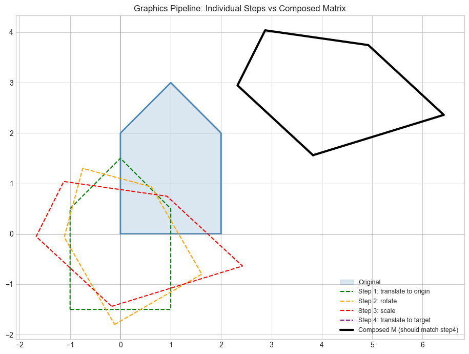
Step-by-step == composed: True
9. Chapter Summary & Connections
Matrix multiplication is function composition:
(AB)v = A(Bv). Apply B first, then A.The formula
C[i,j] = Σ A[i,k]*B[k,j]follows necessarily from the composition requirement.AB ≠ BA in general; order matters.
NumPy’s
@operator calls BLAS routines; scratch implementations are 100-1000x slower.The homogeneous coordinate trick (3×3 matrices for 2D affine transforms) reappears in ch114 (Affine Transformations) and every graphics/robotics application.
Backward connection: This is function composition from ch054 (Function Composition), applied to linear functions.
Forward connections:
In ch157 (Matrix Inverse), we ask: what is the ‘undo’ matrix? The answer requires AB = I.
In ch177 (Linear Algebra for Neural Networks), a forward pass is a chain of matrix multiplications — the computational cost analysis here directly governs model training cost.