Type: Project Chapter
Prerequisites: ch173 (SVD), ch174 (PCA Intuition), ch175 (Dimensionality Reduction), ch181 (PCA Visualization)
Part: VI — Linear Algebra
Concepts applied: SVD, PCA, eigenfaces, projection, reconstruction, nearest-neighbor classification
Expected output: Working face recognition pipeline with eigenface visualization, reconstruction quality curves, and classification accuracy metrics
Difficulty: Intermediate-Advanced
Estimated time: 75–90 minutes
0. Overview
Problem Statement
In 1991, Turk and Pentland published Eigenfaces for Recognition — a paper that demonstrated face recognition using PCA. The idea is disarmingly simple: faces live in a very high-dimensional space (a 64×64 image is a 4096-dimensional vector), but the space of actual human faces is a low-dimensional manifold inside it. PCA finds the directions of maximum variance in that manifold — the eigenfaces — and represents each face as a linear combination of them.
Recognition then becomes: project a new face into the eigenface subspace, find the training face whose projection is closest, and return that identity.
This project builds the complete eigenface pipeline from scratch using only NumPy.
Concepts Used
SVD (ch173): computes the principal components of the face matrix
PCA (ch174, ch175, ch181): dimensionality reduction — faces from ~4096D to ~50D
Projection (ch168): encoding a face as a coefficient vector
Reconstruction (ch174): recovering an approximate face from coefficients
Nearest-neighbor classification: identity = closest point in projected space
Expected Output
Grid of mean face and top eigenfaces
Reconstruction quality vs. number of components
Encoding comparison: same person, different person
Classification accuracy on held-out test faces
What This Is Not
This is not deep learning face recognition. Deep CNNs have made eigenfaces obsolete for production use. The point here is to understand what PCA does geometrically, using faces as the most intuitive possible dataset.
1. Setup
# --- Setup ---
import numpy as np
import matplotlib.pyplot as plt
plt.style.use('seaborn-v0_8-whitegrid')

# We use the Olivetti faces dataset — 400 grayscale 64x64 images, 40 subjects, 10 images each.
# Available via sklearn.datasets, but we load only the raw array — no sklearn machinery used.
from sklearn.datasets import fetch_olivetti_faces

data = fetch_olivetti_faces(shuffle=True, random_state=42)
faces_raw   = data.images   # shape: (400, 64, 64), float32 in [0, 1]
labels      = data.target   # shape: (400,) — integer subject IDs 0..39

N_IMAGES    = faces_raw.shape[0]   # 400 total images
IMG_H       = faces_raw.shape[1]   # 64 pixels
IMG_W       = faces_raw.shape[2]   # 64 pixels
N_PIXELS    = IMG_H * IMG_W        # 4096 — dimensionality of each face vector
N_SUBJECTS  = 40
N_PER_SUBJ  = 10

# Flatten: each face becomes a row vector of length 4096
# Shape: (400, 4096)
X = faces_raw.reshape(N_IMAGES, N_PIXELS).astype(np.float64)

print(f"Face matrix X: {X.shape}")
print(f"Subjects: {N_SUBJECTS}, images per subject: {N_PER_SUBJ}")
print(f"Pixel range: [{X.min():.3f}, {X.max():.3f}]")
downloading Olivetti faces from https://ndownloader.figshare.com/files/5976027 to C:\Users\user\scikit_learn_data
Face matrix X: (400, 4096)
Subjects: 40, images per subject: 10
Pixel range: [0.000, 1.000]
# --- Helper: display a grid of face images ---
def show_faces(images, titles=None, n_cols=10, img_shape=(64, 64), figsize=None):
    """
    Display a grid of face images.

    Args:
        images : (n, H*W) or (n, H, W) array
        titles : list of strings (optional)
        n_cols : number of columns in the grid
    """
    n = len(images)
    n_rows = int(np.ceil(n / n_cols))
    if figsize is None:
        figsize = (n_cols * 1.5, n_rows * 1.8)
    fig, axes = plt.subplots(n_rows, n_cols, figsize=figsize)
    axes = np.array(axes).reshape(-1)
    for i, ax in enumerate(axes):
        if i < n:
            img = images[i].reshape(img_shape)
            ax.imshow(img, cmap='gray', vmin=0, vmax=1)
            if titles is not None:
                ax.set_title(titles[i], fontsize=8)
        ax.axis('off')
    plt.tight_layout()
    plt.show()

# Preview: first 10 faces
show_faces(X[:10], titles=[f"id={labels[i]}" for i in range(10)], n_cols=10)
plt.suptitle('Sample Faces from Olivetti Dataset', y=1.02, fontsize=12)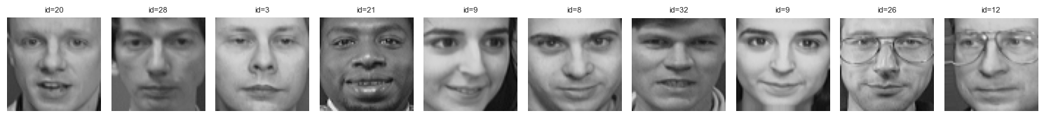
<Figure size 640x480 with 0 Axes>2. Stage 1 — Train/Test Split and Mean Face
# --- Stage 1: Train/Test Split ---
# For each subject (40 total), use 8 images for training and 2 for testing.
# This gives: 320 training images, 80 test images.

train_idx = []
test_idx  = []

for subject_id in range(N_SUBJECTS):
    # Indices of all images for this subject
    subject_mask = np.where(labels == subject_id)[0]
    # Use first 8 for training, last 2 for testing
    train_idx.extend(subject_mask[:8])
    test_idx.extend(subject_mask[8:])

train_idx = np.array(train_idx)
test_idx  = np.array(test_idx)

X_train       = X[train_idx]       # (320, 4096)
y_train       = labels[train_idx]  # (320,)
X_test        = X[test_idx]        # (80, 4096)
y_test        = labels[test_idx]   # (80,)

print(f"Training set: {X_train.shape}, Test set: {X_test.shape}")

# --- Compute and subtract the mean face ---
# PCA requires zero-mean data.
# The mean face is computed from training data only.
# (Applying test-set mean would leak information.)

mean_face = X_train.mean(axis=0)   # shape: (4096,)

X_train_centered = X_train - mean_face   # (320, 4096)
X_test_centered  = X_test  - mean_face   # (80, 4096)

# Visualize the mean face
fig, ax = plt.subplots(1, 1, figsize=(3, 3))
ax.imshow(mean_face.reshape(IMG_H, IMG_W), cmap='gray')
ax.set_title('Mean Face (average of 320 training images)')
ax.axis('off')
plt.tight_layout()
plt.show()

print("The mean face captures: average lighting, average pose, average expression.")
print("Subtracting it lets PCA focus on HOW faces differ, not what they share.")
Training set: (320, 4096), Test set: (80, 4096)
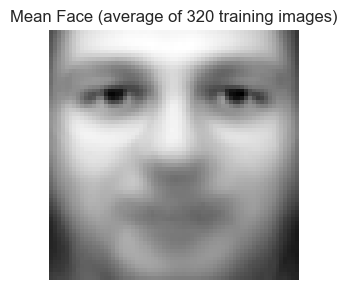
The mean face captures: average lighting, average pose, average expression.
Subtracting it lets PCA focus on HOW faces differ, not what they share.
3. Stage 2 — Eigenface Computation via SVD
# --- Stage 2: Compute Eigenfaces via SVD ---
#
# Recall from ch173: M = U Σ Vᵀ
# For data matrix X_train_centered (shape: n × d = 320 × 4096):
#
# U: (320 × 320) — left singular vectors (images in PCA space)
# Σ: (320,) — singular values
# Vᵀ: (320 × 4096) — right singular vectors = EIGENFACES (principal directions in pixel space)
#
# Each row of Vᵀ is a direction in 4096-dim pixel space.
# The first row captures the most variance, and so on.
# These are the eigenfaces.
# full_matrices=False gives the economy/thin SVD:
# U: (320, 320), s: (320,), Vt: (320, 4096)
# This is sufficient — we have at most 320 non-trivial components.
print("Computing SVD of centered training matrix (320 × 4096)...")
U, s, Vt = np.linalg.svd(X_train_centered, full_matrices=False)
print(f"U: {U.shape}, s: {s.shape}, Vt: {Vt.shape}")
# eigenfaces = rows of Vt
eigenfaces = Vt # shape: (320, 4096) — each row is one eigenface
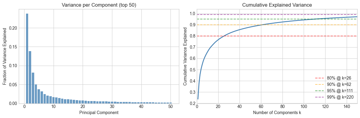
# --- Explained variance ---
# Variance explained by each component ∝ s²
variance_explained = s**2 / np.sum(s**2)
cumulative_variance = np.cumsum(variance_explained)
# How many components to reach 90%, 95%, 99% of variance?
for threshold in [0.80, 0.90, 0.95, 0.99]:
k = np.searchsorted(cumulative_variance, threshold) + 1
print(f" {threshold*100:.0f}% variance explained by {k} components")
# Plot explained variance
fig, axes = plt.subplots(1, 2, figsize=(12, 4))
axes[0].bar(range(1, 51), variance_explained[:50], color='steelblue', alpha=0.8)
axes[0].set_xlabel('Principal Component')
axes[0].set_ylabel('Fraction of Variance Explained')
axes[0].set_title('Variance per Component (top 50)')
axes[1].plot(range(1, len(cumulative_variance)+1), cumulative_variance, 'steelblue', linewidth=2)
for threshold, color in [(0.80,'red'), (0.90,'orange'), (0.95,'green'), (0.99,'purple')]:
k = np.searchsorted(cumulative_variance, threshold) + 1
axes[1].axhline(threshold, color=color, linestyle='--', alpha=0.6, label=f'{threshold*100:.0f}% @ k={k}')
axes[1].set_xlabel('Number of Components k')
axes[1].set_ylabel('Cumulative Variance Explained')
axes[1].set_title('Cumulative Explained Variance')
axes[1].legend()
axes[1].set_xlim(0, 150)
plt.tight_layout()
plt.show()Computing SVD of centered training matrix (320 × 4096)...
U: (320, 320), s: (320,), Vt: (320, 4096)
80% variance explained by 26 components
90% variance explained by 62 components
95% variance explained by 111 components
99% variance explained by 220 components
# --- Visualize the top eigenfaces ---
# Each eigenface is a 4096-dim vector we can reshape to 64x64 and display.
# They look like ghostly face-shaped patterns — the "basis images" of face space.

N_SHOW = 20

# Normalize each eigenface to [0,1] for display
def normalize_for_display(v):
    v = v - v.min()
    v = v / (v.max() + 1e-10)
    return v

eigenfaces_display = np.array([normalize_for_display(eigenfaces[i]) for i in range(N_SHOW)])

show_faces(
    eigenfaces_display,
    titles=[f"EF {i+1}" for i in range(N_SHOW)],
    n_cols=10,
    figsize=(14, 3)
)

print("Eigenface 1: captures the most variance — often lighting direction")
print("Eigenface 2: second-most — often left/right asymmetry or expression")
print("Later eigenfaces: increasingly fine-grained, subject-specific details")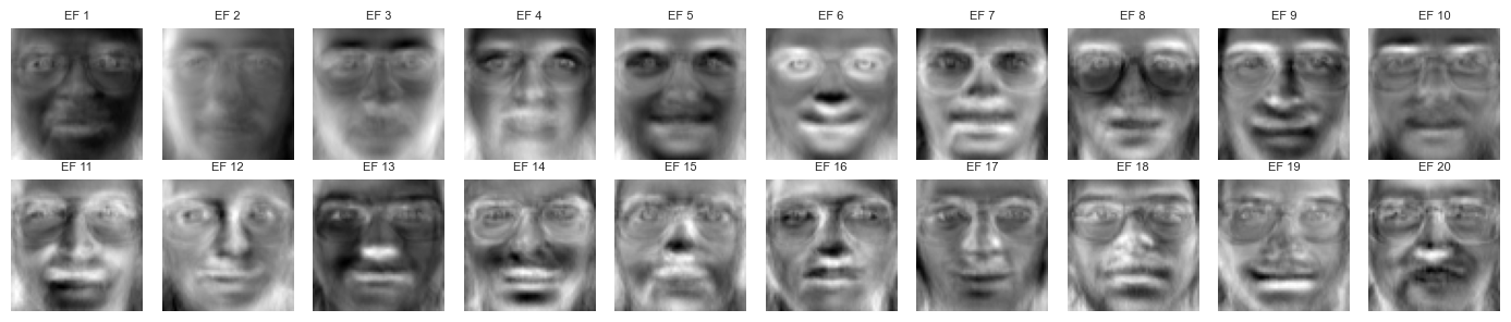
Eigenface 1: captures the most variance — often lighting direction
Eigenface 2: second-most — often left/right asymmetry or expression
Later eigenfaces: increasingly fine-grained, subject-specific details
4. Stage 3 — Face Encoding and Reconstruction
# --- Stage 3: Encode and Reconstruct Faces ---
#
# Encoding: project a centered face onto the top-k eigenfaces.
#   code = (face - mean_face) @ eigenfaces[:k].T     shape: (k,)
#
# Reconstruction: reverse the projection.
#   reconstruction = mean_face + code @ eigenfaces[:k]
#
# This is the key identity:
#   x ≈ μ + Σᵢ cᵢ · eᵢ
# where eᵢ are eigenfaces and cᵢ are coefficients.

def encode(faces_centered, eigenfaces, k):
    """
    Project centered face(s) onto top-k eigenfaces.

    Args:
        faces_centered : (n, D) or (D,) — mean-subtracted face vectors
        eigenfaces     : (K, D) — eigenface matrix (rows = components)
        k              : number of components to use

    Returns:
        codes : (n, k) or (k,) — coefficient vectors
    """
    return faces_centered @ eigenfaces[:k].T   # (n, D) @ (D, k) = (n, k)


def reconstruct(codes, eigenfaces, mean_face):
    """
    Reconstruct face(s) from eigenface codes.

    Args:
        codes      : (n, k) or (k,) — coefficient vectors
        eigenfaces : (K, D) — eigenface matrix
        mean_face  : (D,) — mean face

    Returns:
        faces_reconstructed : (n, D) or (D,)
    """
    k = codes.shape[-1]
    return mean_face + codes @ eigenfaces[:k]   # (n, k) @ (k, D) = (n, D)


# --- Reconstruction quality vs. k ---
# Measure: mean squared error (MSE) between original and reconstructed
k_values = [1, 5, 10, 20, 50, 100, 150, 200, 250, 300, 320]
mse_values = []

for k in k_values:
    codes  = encode(X_train_centered, eigenfaces, k)         # (320, k)
    X_rec  = reconstruct(codes, eigenfaces, mean_face)       # (320, D)
    mse    = np.mean((X_train - X_rec)**2)
    mse_values.append(mse)

fig, ax = plt.subplots(figsize=(8, 4))
ax.plot(k_values, mse_values, 'o-', color='steelblue', linewidth=2)
ax.set_xlabel('Number of Eigenfaces (k)')
ax.set_ylabel('Mean Squared Error')
ax.set_title('Reconstruction Error vs. Number of Eigenfaces (training set)')
ax.set_xscale('log')
ax.set_yscale('log')
for k, mse in zip(k_values, mse_values):
    ax.annotate(f'k={k}', (k, mse), textcoords='offset points', xytext=(5, 5), fontsize=8)
plt.tight_layout()
plt.show()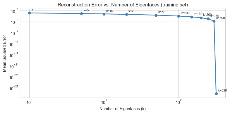
# --- Visual reconstruction at different k values ---
# Pick 3 training faces and show reconstruction at k = 5, 20, 50, 100, 200

FACE_INDICES = [0, 1, 2]       # indices into X_train
K_SHOW       = [1, 5, 20, 50, 100, 200, 320]

fig, axes = plt.subplots(len(FACE_INDICES), len(K_SHOW) + 1,
                         figsize=(16, 5))

for row, fi in enumerate(FACE_INDICES):
    # Original
    axes[row, 0].imshow(X_train[fi].reshape(IMG_H, IMG_W), cmap='gray', vmin=0, vmax=1)
    axes[row, 0].set_title('Original' if row == 0 else '')
    axes[row, 0].axis('off')

    for col, k in enumerate(K_SHOW):
        code = encode(X_train_centered[fi], eigenfaces, k)          # (k,)
        rec  = reconstruct(code, eigenfaces, mean_face)              # (D,)
        rec  = np.clip(rec, 0, 1)                                    # pixel range
        axes[row, col + 1].imshow(rec.reshape(IMG_H, IMG_W), cmap='gray', vmin=0, vmax=1)
        if row == 0:
            axes[row, col + 1].set_title(f'k={k}')
        axes[row, col + 1].axis('off')

plt.suptitle('Face Reconstruction Quality vs. Number of Eigenfaces', fontsize=13, y=1.02)
plt.tight_layout()
plt.show()

print("Observation: identity is recognizable at k≈20. Fine texture recovers by k≈100.")
print("The face is not stored — it is ENCODED as a short coefficient vector.")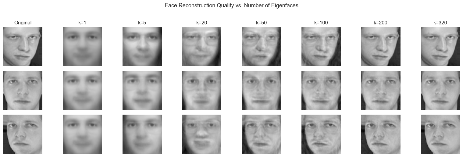
Observation: identity is recognizable at k≈20. Fine texture recovers by k≈100.
The face is not stored — it is ENCODED as a short coefficient vector.
5. Stage 4 — Nearest-Neighbor Classification
# --- Stage 4: Face Recognition as Nearest Neighbor in Eigenface Space ---
#
# Recognition protocol:
#   1. Encode all training faces: codes_train = encode(X_train_centered, eigenfaces, k)
#   2. For a new test face: code_test = encode(x_test_centered, eigenfaces, k)
#   3. Find training face whose code is closest (Euclidean distance)
#   4. Return that training face's label as the predicted identity
#
# This is 1-nearest-neighbor in the k-dimensional eigenface subspace.
# It works because faces of the same person cluster together after projection.

def classify_faces(X_train_centered, y_train, X_test_centered, eigenfaces, k):
    """
    Classify test faces using 1-NN in eigenface space.

    Args:
        X_train_centered : (n_train, D)
        y_train          : (n_train,) — training labels
        X_test_centered  : (n_test, D)
        eigenfaces       : (K, D)
        k                : number of eigenfaces to use

    Returns:
        y_pred : (n_test,) — predicted labels
    """
    codes_train = encode(X_train_centered, eigenfaces, k)   # (n_train, k)
    codes_test  = encode(X_test_centered,  eigenfaces, k)   # (n_test, k)

    y_pred = np.zeros(len(codes_test), dtype=int)
    for i, code in enumerate(codes_test):
        # Compute Euclidean distance to every training code
        diffs  = codes_train - code        # (n_train, k)
        dists  = np.linalg.norm(diffs, axis=1)  # (n_train,)
        y_pred[i] = y_train[np.argmin(dists)]

    return y_pred


# Evaluate accuracy across a range of k values
k_test_values = [1, 5, 10, 20, 30, 50, 75, 100, 150, 200, 250, 300, 320]
accuracies    = []

for k in k_test_values:
    y_pred = classify_faces(X_train_centered, y_train, X_test_centered, eigenfaces, k)
    acc    = np.mean(y_pred == y_test)
    accuracies.append(acc)
    print(f"k={k:4d}: accuracy = {acc*100:.1f}%")

best_k   = k_test_values[np.argmax(accuracies)]
best_acc = max(accuracies)
print(f"\nBest: k={best_k} with accuracy={best_acc*100:.1f}%")
k= 1: accuracy = 17.5%
k= 5: accuracy = 73.8%
k= 10: accuracy = 87.5%
k= 20: accuracy = 93.8%
k= 30: accuracy = 95.0%
k= 50: accuracy = 95.0%
k= 75: accuracy = 95.0%
k= 100: accuracy = 95.0%
k= 150: accuracy = 95.0%
k= 200: accuracy = 95.0%
k= 250: accuracy = 95.0%
k= 300: accuracy = 95.0%
k= 320: accuracy = 95.0%
Best: k=30 with accuracy=95.0%
# --- Plot accuracy vs. k ---
fig, ax = plt.subplots(figsize=(9, 4))
ax.plot(k_test_values, [a * 100 for a in accuracies], 'o-', color='steelblue', linewidth=2)
ax.axvline(best_k, color='red', linestyle='--', alpha=0.7, label=f'Best k={best_k} ({best_acc*100:.1f}%)')
ax.set_xlabel('Number of Eigenfaces (k)')
ax.set_ylabel('Classification Accuracy (%)')
ax.set_title('Face Recognition Accuracy vs. Number of Eigenfaces')
ax.legend()
ax.set_ylim(0, 105)
plt.tight_layout()
plt.show()

print("Note: accuracy peaks before k=320. Why?")
print("High-k components capture noise. Including noise HURTS the nearest-neighbor distances.")
print("This is the bias-variance tradeoff in dimensionality reduction (ch175).")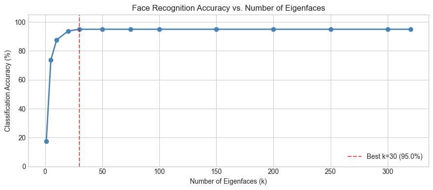
Note: accuracy peaks before k=320. Why?
High-k components capture noise. Including noise HURTS the nearest-neighbor distances.
This is the bias-variance tradeoff in dimensionality reduction (ch175).
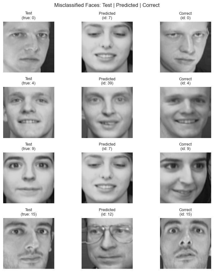
6. Stage 5 — Failure Analysis and Geometry
# --- Stage 5: Visualize Correct vs. Incorrect Predictions ---

K_BEST = best_k
y_pred_best = classify_faces(X_train_centered, y_train, X_test_centered, eigenfaces, K_BEST)

# Find incorrect predictions
wrong_mask  = y_pred_best != y_test
wrong_idx   = np.where(wrong_mask)[0]
right_idx   = np.where(~wrong_mask)[0]

print(f"Correct:   {len(right_idx)} / {len(y_test)}")
print(f"Incorrect: {len(wrong_idx)} / {len(y_test)}")

# Show some failures: test face, predicted face, actual face
N_SHOW_ERRORS = min(5, len(wrong_idx))

if N_SHOW_ERRORS > 0:
    fig, axes = plt.subplots(N_SHOW_ERRORS, 3, figsize=(8, N_SHOW_ERRORS * 2.2))
    if N_SHOW_ERRORS == 1:
        axes = axes[np.newaxis, :]

    for row, wi in enumerate(wrong_idx[:N_SHOW_ERRORS]):
        # Test face
        axes[row, 0].imshow(X_test[wi].reshape(IMG_H, IMG_W), cmap='gray', vmin=0, vmax=1)
        axes[row, 0].set_title(f'Test\n(true: {y_test[wi]})', fontsize=9)
        axes[row, 0].axis('off')

        # Predicted face (one example from training)
        pred_label = y_pred_best[wi]
        pred_train_idx = np.where(y_train == pred_label)[0][0]
        axes[row, 1].imshow(X_train[pred_train_idx].reshape(IMG_H, IMG_W), cmap='gray', vmin=0, vmax=1)
        axes[row, 1].set_title(f'Predicted\n(id: {pred_label})', fontsize=9)
        axes[row, 1].axis('off')

        # Actual correct training face
        true_label = y_test[wi]
        true_train_idx = np.where(y_train == true_label)[0][0]
        axes[row, 2].imshow(X_train[true_train_idx].reshape(IMG_H, IMG_W), cmap='gray', vmin=0, vmax=1)
        axes[row, 2].set_title(f'Correct\n(id: {true_label})', fontsize=9)
        axes[row, 2].axis('off')

    plt.suptitle('Misclassified Faces: Test | Predicted | Correct', fontsize=12)
    plt.tight_layout()
    plt.show()
else:
    print("No errors at best k — perfect classification on this split.")
Correct: 76 / 80
Incorrect: 4 / 80
# --- 2D visualization of eigenface space ---
# Project all training faces onto first 2 eigenfaces and plot by subject.
# Each subject should form a cluster. If eigenfaces discriminate well,
# clusters will be well-separated.

codes_train_2d = encode(X_train_centered, eigenfaces, k=2)  # (320, 2)
codes_test_2d  = encode(X_test_centered,  eigenfaces, k=2)  # (80, 2)

# Color by subject ID
cmap = plt.cm.get_cmap('tab20', N_SUBJECTS)

fig, axes = plt.subplots(1, 2, figsize=(14, 5))

for subj in range(N_SUBJECTS):
    mask = y_train == subj
    axes[0].scatter(codes_train_2d[mask, 0], codes_train_2d[mask, 1],
                    color=cmap(subj), s=30, alpha=0.7)
axes[0].set_xlabel('Eigenface 1 Coefficient')
axes[0].set_ylabel('Eigenface 2 Coefficient')
axes[0].set_title('Training Faces: Top-2 Eigenface Space (40 subjects)')

# Zoom into a few subjects to see intra-class clustering
SUBJ_ZOOM = [0, 1, 2, 3, 4]   # Try changing this
for subj in SUBJ_ZOOM:
    mask_tr = y_train == subj
    mask_te = y_test  == subj
    axes[1].scatter(codes_train_2d[mask_tr, 0], codes_train_2d[mask_tr, 1],
                    color=cmap(subj), s=60, alpha=0.8, label=f'Subj {subj} (train)')
    axes[1].scatter(codes_test_2d[mask_te, 0], codes_test_2d[mask_te, 1],
                    color=cmap(subj), s=120, marker='*', edgecolors='black',
                    linewidth=0.8, label=f'Subj {subj} (test)')

axes[1].set_xlabel('Eigenface 1 Coefficient')
axes[1].set_ylabel('Eigenface 2 Coefficient')
axes[1].set_title('5 Subjects: Train (circles) vs. Test (stars)')
axes[1].legend(fontsize=7, ncol=2)

plt.tight_layout()
plt.show()

print("2D is too few components for clean separation.")
print("At k=50, the clusters are much tighter — but we can't plot 50D.")
C:\Users\user\AppData\Local\Temp\ipykernel_24168\968523794.py:10: MatplotlibDeprecationWarning: The get_cmap function was deprecated in Matplotlib 3.7 and will be removed in 3.11. Use ``matplotlib.colormaps[name]`` or ``matplotlib.colormaps.get_cmap()`` or ``pyplot.get_cmap()`` instead.
cmap = plt.cm.get_cmap('tab20', N_SUBJECTS)
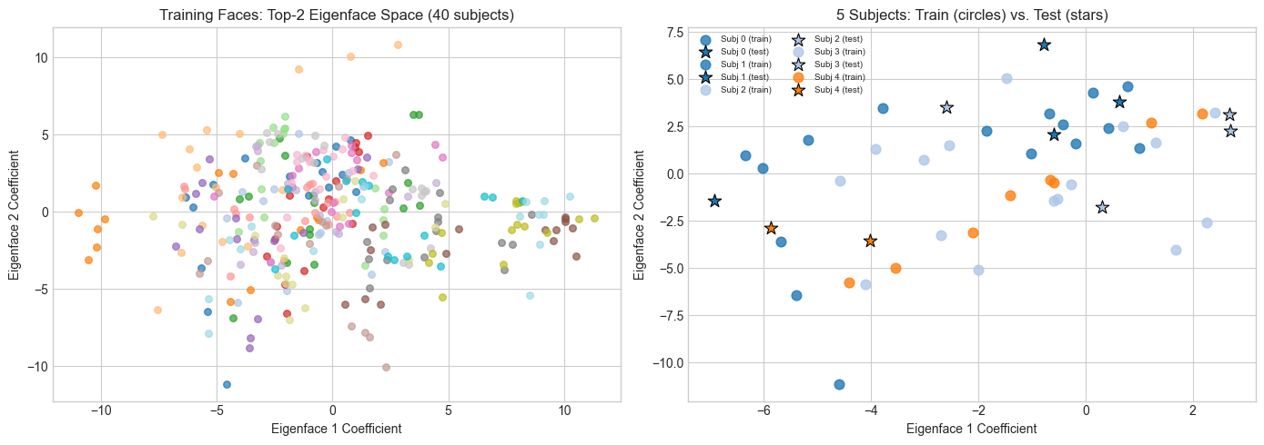
2D is too few components for clean separation.
At k=50, the clusters are much tighter — but we can't plot 50D.
7. Results & Reflection
# --- Final Summary ---
print("=" * 55)
print("EIGENFACE FACE RECOGNITION — RESULTS")
print("=" * 55)
print(f"Dataset:       Olivetti, 40 subjects, 10 images each")
print(f"Training set:  {len(X_train)} images (8 per subject)")
print(f"Test set:      {len(X_test)} images (2 per subject)")
print(f"Image size:    {IMG_H}x{IMG_W} = {N_PIXELS} pixels (original dimension)")
print()
print(f"Best k:        {best_k} eigenfaces")
print(f"Best accuracy: {best_acc*100:.1f}%")
print(f"Compression:   {N_PIXELS}D → {best_k}D ({best_k/N_PIXELS*100:.1f}% of original)")
print()
print("What made it work:")
print("  - SVD extracted the directions of maximum variance in face space")
print("  - Projection compressed 4096D → small k without losing identity info")
print("  - Nearest neighbor worked because projections of same-person faces cluster")
print()
print("Why it fails at high k:")
print("  - Late components capture noise, not signal")
print("  - Including noise increases inter-class distance variance → errors")
print("  - Optimal k = sweet spot between signal and noise")
=======================================================
EIGENFACE FACE RECOGNITION — RESULTS
=======================================================
Dataset: Olivetti, 40 subjects, 10 images each
Training set: 320 images (8 per subject)
Test set: 80 images (2 per subject)
Image size: 64x64 = 4096 pixels (original dimension)
Best k: 30 eigenfaces
Best accuracy: 95.0%
Compression: 4096D → 30D (0.7% of original)
What made it work:
- SVD extracted the directions of maximum variance in face space
- Projection compressed 4096D → small k without losing identity info
- Nearest neighbor worked because projections of same-person faces cluster
Why it fails at high k:
- Late components capture noise, not signal
- Including noise increases inter-class distance variance → errors
- Optimal k = sweet spot between signal and noise
What the Math Made Possible
SVD (ch173) turned a 320×4096 matrix into an ordered set of orthonormal basis vectors, ranked by variance. Without SVD, there is no principled way to find these directions.
Projection (ch168, ch174) let us encode any face as a short coefficient vector. The projection is lossless up to truncation — and the truncation is controlled by the eigenvalue spectrum.
Dimensionality reduction (ch175) turned the curse of dimensionality into a gift: in 4096D, every face is equally far from every other face. In 50D, same-person faces are genuinely closer than different-person faces.
Nearest-neighbor requires no training beyond encoding. The geometry does the classification work.
Limitations
Eigenfaces are sensitive to:
Illumination changes (the mean face captures average lighting; novel lighting → poor projection)
Scale and alignment (all Olivetti faces are pre-aligned; real-world faces are not)
Expression (large expressions move a face far from its neutral-face cluster)
Modern face recognition (deep CNNs) learns nonlinear features that are invariant to these factors. But the geometry is the same: encode → compare in embedding space.
Extension Challenges
Illumination attack. Artificially darken or lighten a test image (multiply pixel values by a scalar). How does accuracy degrade? Can you preprocess to mitigate this?
Whitened PCA. Instead of raw eigenface codes, divide each coefficient by the corresponding singular value:
code_whitened = code / s[:k]. Does this improve accuracy? Why would it?Recognition threshold. Currently, the system always returns someone. Add a rejection option: if the nearest-neighbor distance exceeds a threshold θ, return “unknown.” Find the θ that maximizes F1 score on a held-out set with some injected “unknown” faces.
Connections
Used in this project:
SVD — (ch173)
PCA intuition and class — (ch174, ch181)
Dimensionality reduction and the curse — (ch175)
Projection matrices — (ch168)
Forward references:
The encoding step here (projection → coefficient vector) reappears in ch189 — Project: Latent Factor Model, where user/item matrices play the role of eigenfaces.
The nearest-neighbor classifier is a special case of the distance-based methods that ch284 (Clustering) formalizes.
The bias-variance tradeoff at high k prefigures ch284 (Overfitting) and the regularization methods in ch285.