Part VII: Calculus
1. The Starting Point: Average Rate of Change
Before derivatives, there is a simpler question: how fast did something change over an interval?
If a car travels 120 km in 2 hours, its average speed is 60 km/h. This is the average rate of change of position with respect to time.
This is just the slope of the line connecting two points on the graph of f — the secant line.
Calculus asks: what happens when the interval shrinks to zero? The average rate becomes the instantaneous rate. That is the derivative.
(This chapter builds the bridge. Derivatives arrive in ch205.)
import numpy as np
import matplotlib.pyplot as plt

# Position function: s(t) = t^2  (imagine falling object, ignoring sign)
s = lambda t: t**2

t_vals = np.linspace(0, 3, 300)

fig, axes = plt.subplots(1, 2, figsize=(13, 5))

# Left: secant lines shrinking toward tangent
t0 = 1.5
axes[0].plot(t_vals, s(t_vals), color='steelblue', linewidth=2.5, label='s(t) = t²')
axes[0].scatter([t0], [s(t0)], color='red', zorder=6, s=60)

colors = ['#ff9999', '#ff6666', '#cc0000', '#660000']
for h, color in zip([1.0, 0.5, 0.2, 0.05], colors):
    t1 = t0 + h
    slope = (s(t1) - s(t0)) / h
    x_line = np.array([t0 - 0.5, t1 + 0.2])
    y_line = s(t0) + slope * (x_line - t0)
    axes[0].plot(x_line, y_line, color=color, linewidth=1.5, linestyle='--',
                 label=f'h={h}, slope={slope:.3f}')

# True tangent: derivative of t^2 at t0 is 2*t0
true_slope = 2 * t0
x_tan = np.array([t0 - 0.8, t0 + 0.8])
y_tan = s(t0) + true_slope * (x_tan - t0)
axes[0].plot(x_tan, y_tan, color='black', linewidth=2, label=f'tangent slope={true_slope:.3f}')

axes[0].set_xlim(0, 3)
axes[0].set_ylim(-0.5, 9)
axes[0].set_title('Secant lines → tangent line as h → 0')
axes[0].set_xlabel('t')
axes[0].set_ylabel('s(t)')
axes[0].legend(fontsize=8)

# Right: average rate of change vs interval size
h_vals = np.logspace(-3, 0.3, 200)
avg_rates = [(s(t0 + h) - s(t0)) / h for h in h_vals]
axes[1].semilogx(h_vals, avg_rates, color='steelblue', linewidth=2)
axes[1].axhline(y=true_slope, color='red', linestyle='--', label=f'true slope = {true_slope}')
axes[1].set_xlabel('interval size h')
axes[1].set_ylabel('average rate of change')
axes[1].set_title('Average rate converges to instantaneous rate')
axes[1].legend()

plt.suptitle('From Average to Instantaneous Rate of Change', fontsize=13, fontweight='bold')
plt.tight_layout()
plt.show()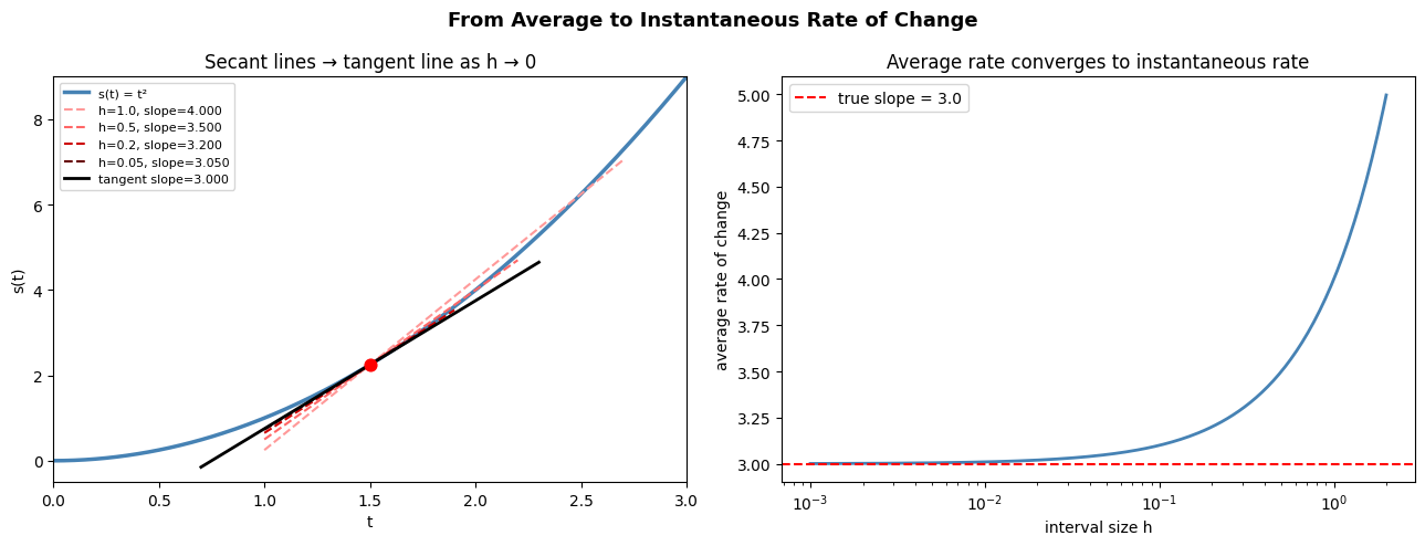
2. Position, Velocity, Acceleration
The classic physical example is motion along a line:
Position s(t): where the object is at time t
Velocity v(t) = s’(t): how fast position changes
Acceleration a(t) = v’(t) = s’'(t): how fast velocity changes
Each is the derivative of the previous. This chain — position → velocity → acceleration — is the simplest example of repeated differentiation (which reappears in ch217 — Second Derivatives).
# Simulate a ball thrown upward: s(t) = v0*t - (1/2)*g*t^2
g = 9.81   # m/s^2
v0 = 20.0  # initial velocity m/s

s_fn  = lambda t: v0 * t - 0.5 * g * t**2          # position
v_fn  = lambda t: v0 - g * t                         # velocity (first derivative)
a_fn  = lambda t: -g * np.ones_like(t)               # acceleration (second derivative)

# Time until ball hits ground: s=0 => t=0 or t=2*v0/g
t_end = 2 * v0 / g
t = np.linspace(0, t_end, 300)

fig, axes = plt.subplots(3, 1, figsize=(10, 9), sharex=True)

axes[0].plot(t, s_fn(t), color='steelblue', linewidth=2)
axes[0].set_ylabel('Position s(t) [m]')
axes[0].set_title('Projectile motion: position')
axes[0].axhline(0, color='gray', linewidth=0.8)
t_peak = v0 / g
axes[0].axvline(t_peak, color='red', linestyle='--', alpha=0.7, label=f'peak at t={t_peak:.2f}s')
axes[0].legend()

axes[1].plot(t, v_fn(t), color='darkorange', linewidth=2)
axes[1].set_ylabel('Velocity v(t) [m/s]')
axes[1].set_title("Velocity = s'(t) — zero at peak")
axes[1].axhline(0, color='gray', linewidth=0.8)
axes[1].axvline(t_peak, color='red', linestyle='--', alpha=0.7)

axes[2].plot(t, a_fn(t), color='green', linewidth=2)
axes[2].set_ylabel('Acceleration a(t) [m/s²]')
axes[2].set_title("Acceleration = v'(t) = -g (constant)")
axes[2].set_xlabel('Time t [s]')
axes[2].axhline(0, color='gray', linewidth=0.8)

plt.tight_layout()
plt.show()

print(f'Peak height: {s_fn(t_peak):.2f} m at t = {t_peak:.2f} s')
print(f'Velocity at peak: {v_fn(t_peak):.4f} m/s (≈ 0, as expected)')
print(f'Acceleration is constant: {a_fn(np.array([0.0]))[0]} m/s² (gravity)')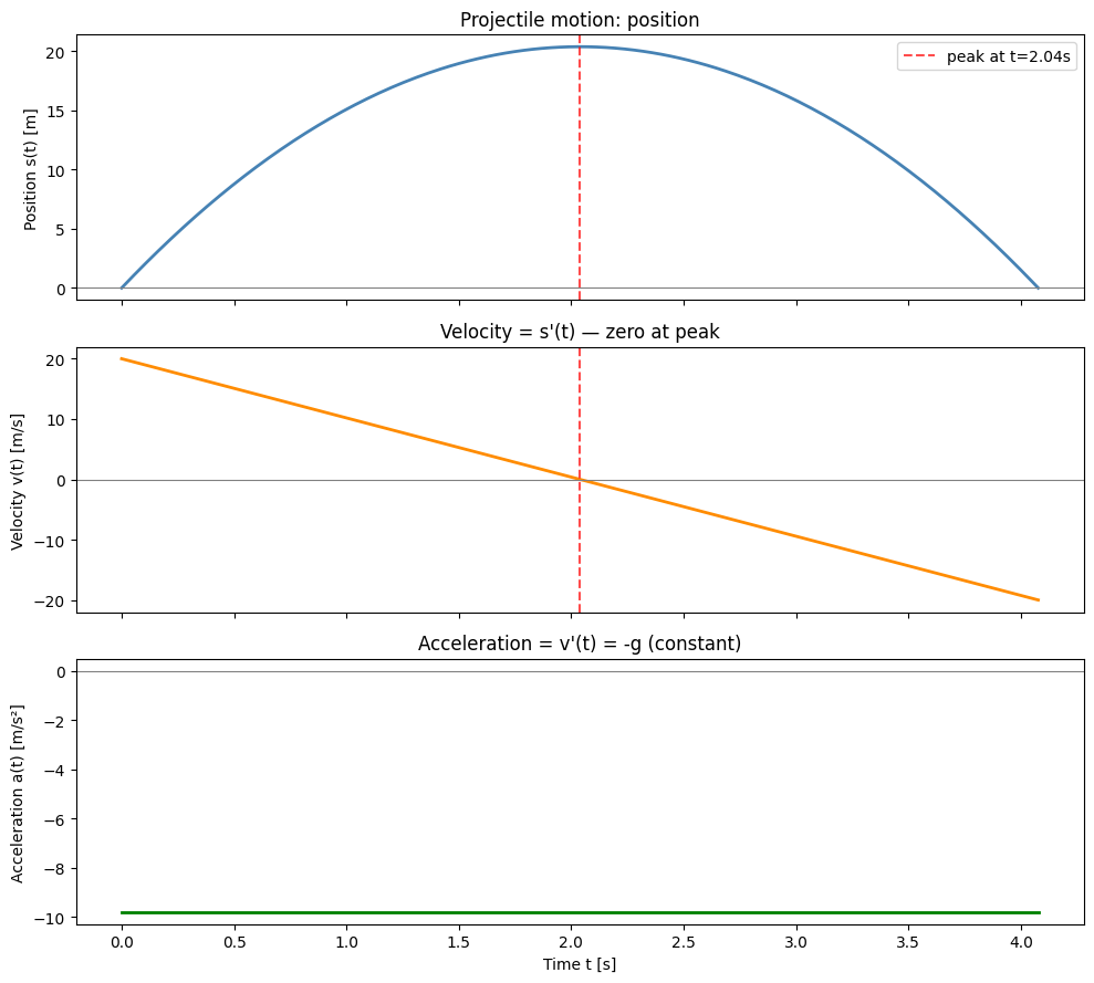
Peak height: 20.39 m at t = 2.04 s
Velocity at peak: 0.0000 m/s (≈ 0, as expected)
Acceleration is constant: -9.81 m/s² (gravity)
3. Numerical Average Rate of Change
You can compute average rates of change on discrete data — no calculus required. This is how NumPy’s np.diff works.
# Loss curve from a training run (simulated)
np.random.seed(0)
steps = np.arange(50)
loss = 2.5 * np.exp(-0.08 * steps) + 0.1 * np.random.randn(50) * np.exp(-0.04 * steps) + 0.15

# Average rate of change between consecutive steps
delta_loss = np.diff(loss)   # loss[i+1] - loss[i]
delta_step = 1               # steps are spaced 1 apart
rate = delta_loss / delta_step

fig, axes = plt.subplots(2, 1, figsize=(10, 7), sharex=True)

axes[0].plot(steps, loss, 'o-', color='steelblue', markersize=3, linewidth=1.5)
axes[0].set_ylabel('Loss')
axes[0].set_title('Training loss curve')

axes[1].bar(steps[:-1], rate, color=np.where(rate < 0, 'steelblue', 'salmon'), alpha=0.8, width=0.8)
axes[1].axhline(0, color='black', linewidth=0.8)
axes[1].set_ylabel('Δloss / Δstep')
axes[1].set_xlabel('Training step')
axes[1].set_title('Rate of change of loss (negative = loss decreasing = good)')

plt.tight_layout()
plt.show()

print(f'Average rate of change across all steps: {np.mean(rate):.5f}')
print(f'This is: (final_loss - initial_loss) / total_steps = ({loss[-1]:.3f} - {loss[0]:.3f}) / 49 = {(loss[-1]-loss[0])/49:.5f}')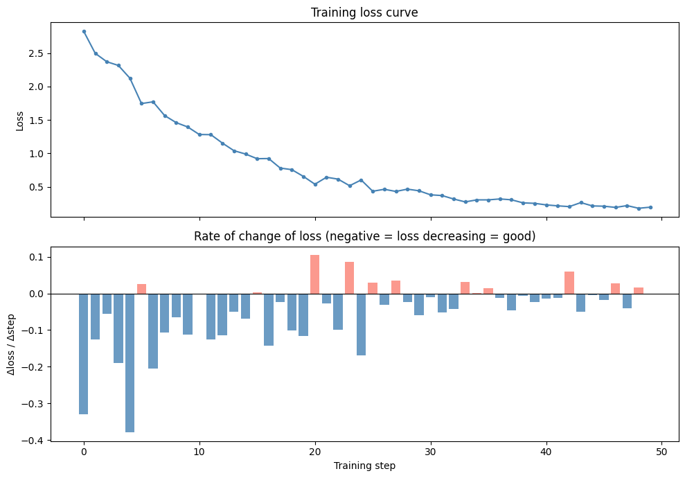
Average rate of change across all steps: -0.05367
This is: (final_loss - initial_loss) / total_steps = (0.197 - 2.826) / 49 = -0.05367
4. Key Vocabulary
| Term | Meaning |
|---|---|
| Secant line | Line through two points on a curve — its slope is the average rate of change |
| Tangent line | Line touching the curve at one point — its slope is the instantaneous rate |
| Difference quotient | [f(x+h) - f(x)] / h — the secant slope formula |
| Derivative | Limit of the difference quotient as h → 0 |
| Rate of change | How much output changes per unit of input change |
5. Summary
Average rate of change = slope of secant line = Δf / Δx
As the interval shrinks, the secant approaches the tangent
The instantaneous rate of change at a point is the derivative
Position → velocity → acceleration is the chain of repeated differentiation
On discrete data,
np.diffgives the finite difference approximation to the derivative
6. Forward References
The difference quotient [f(x+h) - f(x)] / h is formalized as the limit definition of the derivative in ch203 — Limits Intuition and ch205 — Derivative Concept. The chain position → velocity → acceleration reappears in ch217 — Second Derivatives, and again in ch225 — Differential Equations where motion is defined by the equation s’’ = -g.